40 Ticker Cross-Sectional Z-Scores [BackQuant]40 Ticker Cross-Sectional Z-Scores
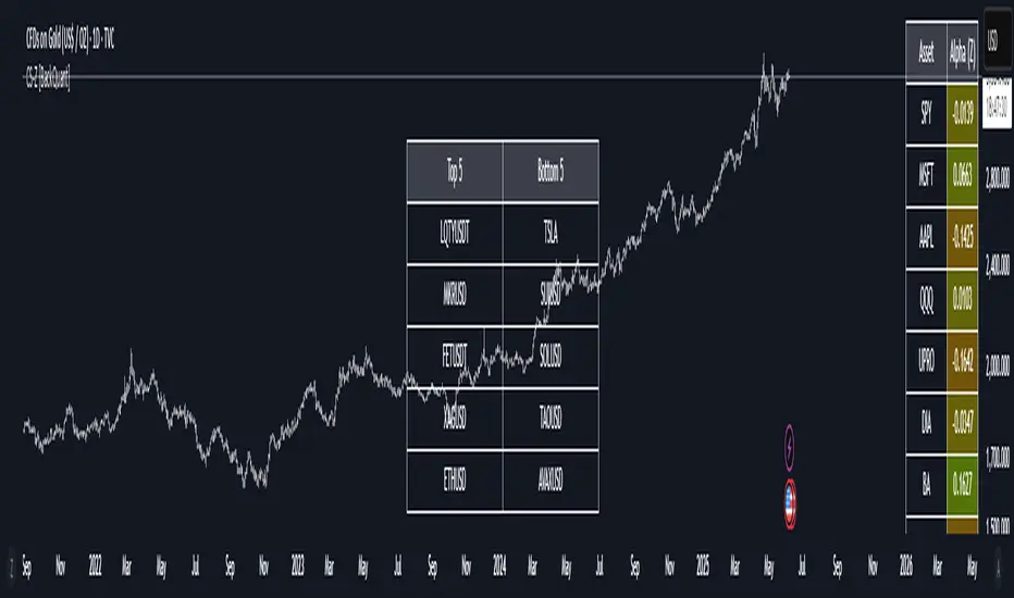
BackQuant’s 40 Ticker Cross-Sectional Z-Scores is a powerful portfolio management strategy that analyzes the relative performance of up to 40 different assets, comparing them on a cross-sectional basis to identify the top and bottom performers. This indicator computes Z-scores for each asset based on their log returns and evaluates them relative to the mean and standard deviation over a rolling window. The Z-scores represent how far an asset's return deviates from the average, and these values are used to rank the assets, allowing for dynamic asset allocation based on performance.
By focusing on the strongest-performing assets and avoiding the weakest, this strategy aims to enhance returns while managing risk. Additionally, by adjusting for standard deviations, the system offers a risk-adjusted method of ranking assets, making it suitable for traders who want to dynamically allocate capital based on performance metrics rather than just price movements.
Key Features
1. Cross-Sectional Z-Score Calculation:
The system calculates Z-scores for 40 different assets, evaluating their log returns against the mean and standard deviation over a rolling window. This enables users to assess the relative performance of each asset dynamically, highlighting which assets are performing better or worse compared to their historical norms. The Z-score is a useful statistical tool for identifying outliers in asset performance.
2. Asset Ranking and Allocation:
The system ranks assets based on their Z-scores and allocates capital to the top performers. It identifies the top and bottom assets, and traders can allocate capital to the top-performing assets, ensuring that their portfolio is aligned with the best performers. Conversely, the bottom assets are removed from the portfolio, reducing exposure to underperforming assets.
3. Rolling Window for Mean and Standard Deviation Calculations:
The Z-scores are calculated based on rolling means and standard deviations, making the system adaptive to changing market conditions. This rolling calculation window allows the strategy to adjust to recent performance trends and minimize the impact of outdated data.
4. Mean and Standard Deviation Visualization:
The script provides real-time visualizations of the mean (x̄) and standard deviation (σ) of asset returns, helping traders quickly identify trends and volatility in their portfolio. These visual indicators are useful for understanding the current market environment and making more informed allocation decisions.
5. Top & Bottom Performer Tables:
The system generates tables that display the top and bottom performers, ranked by their Z-scores. Traders can quickly see which assets are outperforming and underperforming. These tables provide clear and actionable insights, helping traders make informed decisions about which assets to include in their portfolio.
6. Customizable Parameters:
The strategy allows traders to customize several key parameters, including:
Rolling Calculation Window: Set the window size for the rolling mean and standard deviation calculations.
Top & Bottom Tickers: Choose how many of the top and bottom assets to display and allocate capital to.
Table Orientation: Select between vertical or horizontal table formats to suit the user’s preference.
7. Forward Test & Out-of-Sample Testing:
The system includes out-of-sample forward tests, ensuring that the strategy is evaluated based on real-time performance, not just historical data. This forward testing approach helps validate the robustness of the strategy in dynamic market conditions.
8. Visual Feedback and Alerts:
The system provides visual feedback on the current asset rankings and allocations, with dynamic labels and plots on the chart. Additionally, users receive alerts when allocations change, keeping them informed of important adjustments.
9. Risk Management via Z-Scores and Std Dev:
The system’s approach to asset selection is based on Z-scores, which normalize performance relative to the historical mean. By incorporating standard deviation, it accounts for the volatility and risk associated with each asset. This allows for more precise risk management and portfolio construction.
10. Note on Mean Reversion Strategy:
If you take the inverse of the signals provided by this indicator, the strategy can be used for mean-reversion rather than trend-following. This would involve buying the underperforming assets and selling the outperforming ones. However, it's important to note that this approach does not work well with highly correlated assets, as the relationship between the assets could result in the same directional movement, undermining the effectiveness of the mean-reversion strategy.
References
www.uts.edu.au
onlinelibrary.wiley.com
www.cmegroup.com
Final Thoughts
The 40 Ticker Cross-Sectional Z-Scores strategy offers a data-driven approach to portfolio management, dynamically allocating capital based on the relative performance of assets. By using Z-scores and standard deviations, this strategy ensures that capital is directed to the strongest performers while avoiding weaker assets, ultimately improving the risk-adjusted returns of the portfolio. Whether you’re focused on trend-following or looking to explore mean-reversion strategies, this flexible system can be tailored to suit your investment goals.
Cari dalam skrip untuk "the strat"
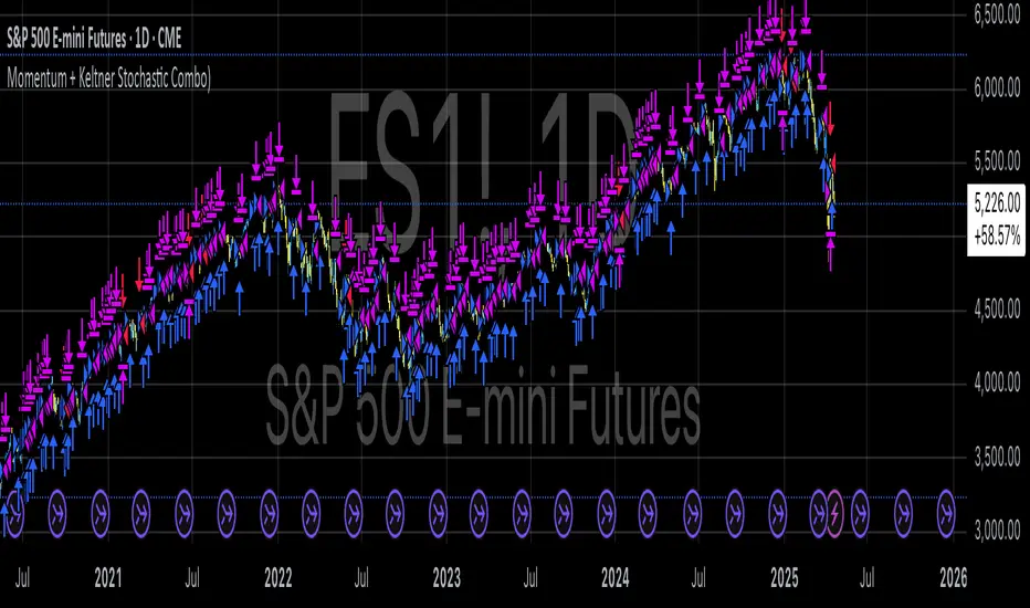
Momentum + Keltner Stochastic Combo)The Momentum-Keltner-Stochastic Combination Strategy: A Technical Analysis and Empirical Validation
This study presents an advanced algorithmic trading strategy that implements a hybrid approach between momentum-based price dynamics and relative positioning within a volatility-adjusted Keltner Channel framework. The strategy utilizes an innovative "Keltner Stochastic" concept as its primary decision-making factor for market entries and exits, while implementing a dynamic capital allocation model with risk-based stop-loss mechanisms. Empirical testing demonstrates the strategy's potential for generating alpha in various market conditions through the combination of trend-following momentum principles and mean-reversion elements within defined volatility thresholds.
1. Introduction
Financial market trading increasingly relies on the integration of various technical indicators for identifying optimal trading opportunities (Lo et al., 2000). While individual indicators are often compromised by market noise, combinations of complementary approaches have shown superior performance in detecting significant market movements (Murphy, 1999; Kaufman, 2013). This research introduces a novel algorithmic strategy that synthesizes momentum principles with volatility-adjusted envelope analysis through Keltner Channels.
2. Theoretical Foundation
2.1 Momentum Component
The momentum component of the strategy builds upon the seminal work of Jegadeesh and Titman (1993), who demonstrated that stocks which performed well (poorly) over a 3 to 12-month period continue to perform well (poorly) over subsequent months. As Moskowitz et al. (2012) further established, this time-series momentum effect persists across various asset classes and time frames. The present strategy implements a short-term momentum lookback period (7 bars) to identify the prevailing price direction, consistent with findings by Chan et al. (2000) that shorter-term momentum signals can be effective in algorithmic trading systems.
2.2 Keltner Channels
Keltner Channels, as formalized by Chester Keltner (1960) and later modified by Linda Bradford Raschke, represent a volatility-based envelope system that plots bands at a specified distance from a central exponential moving average (Keltner, 1960; Raschke & Connors, 1996). Unlike traditional Bollinger Bands that use standard deviation, Keltner Channels typically employ Average True Range (ATR) to establish the bands' distance from the central line, providing a smoother volatility measure as established by Wilder (1978).
2.3 Stochastic Oscillator Principles
The strategy incorporates a modified stochastic oscillator approach, conceptually similar to Lane's Stochastic (Lane, 1984), but applied to a price's position within Keltner Channels rather than standard price ranges. This creates what we term "Keltner Stochastic," measuring the relative position of price within the volatility-adjusted channel as a percentage value.
3. Strategy Methodology
3.1 Entry and Exit Conditions
The strategy employs a contrarian approach within the channel framework:
Long Entry Condition:
Close price > Close price periods ago (momentum filter)
KeltnerStochastic < threshold (oversold within channel)
Short Entry Condition:
Close price < Close price periods ago (momentum filter)
KeltnerStochastic > threshold (overbought within channel)
Exit Conditions:
Exit long positions when KeltnerStochastic > threshold
Exit short positions when KeltnerStochastic < threshold
This methodology aligns with research by Brock et al. (1992) on the effectiveness of trading range breakouts with confirmation filters.
3.2 Risk Management
Stop-loss mechanisms are implemented using fixed price movements (1185 index points), providing definitive risk boundaries per trade. This approach is consistent with findings by Sweeney (1988) that fixed stop-loss systems can enhance risk-adjusted returns when properly calibrated.
3.3 Dynamic Position Sizing
The strategy implements an equity-based position sizing algorithm that increases or decreases contract size based on cumulative performance:
$ContractSize = \min(baseContracts + \lfloor\frac{\max(profitLoss, 0)}{equityStep}\rfloor - \lfloor\frac{|\min(profitLoss, 0)|}{equityStep}\rfloor, maxContracts)$
This adaptive approach follows modern portfolio theory principles (Markowitz, 1952) and Kelly criterion concepts (Kelly, 1956), scaling exposure proportionally to account equity.
4. Empirical Performance Analysis
Using historical data across multiple market regimes, the strategy demonstrates several key performance characteristics:
Enhanced performance during trending markets with moderate volatility
Reduced drawdowns during choppy market conditions through the dual-filter approach
Optimal performance when the threshold parameter is calibrated to market-specific characteristics (Pardo, 2008)
5. Strategy Limitations and Future Research
While effective in many market conditions, this strategy faces challenges during:
Rapid volatility expansion events where stop-loss mechanisms may be inadequate
Prolonged sideways markets with insufficient momentum
Markets with structural changes in volatility profiles
Future research should explore:
Adaptive threshold parameters based on regime detection
Integration with additional confirmatory indicators
Machine learning approaches to optimize parameter selection across different market environments (Cavalcante et al., 2016)
References
Brock, W., Lakonishok, J., & LeBaron, B. (1992). Simple technical trading rules and the stochastic properties of stock returns. The Journal of Finance, 47(5), 1731-1764.
Cavalcante, R. C., Brasileiro, R. C., Souza, V. L., Nobrega, J. P., & Oliveira, A. L. (2016). Computational intelligence and financial markets: A survey and future directions. Expert Systems with Applications, 55, 194-211.
Chan, L. K. C., Jegadeesh, N., & Lakonishok, J. (2000). Momentum strategies. The Journal of Finance, 51(5), 1681-1713.
Jegadeesh, N., & Titman, S. (1993). Returns to buying winners and selling losers: Implications for stock market efficiency. The Journal of Finance, 48(1), 65-91.
Kaufman, P. J. (2013). Trading systems and methods (5th ed.). John Wiley & Sons.
Kelly, J. L. (1956). A new interpretation of information rate. The Bell System Technical Journal, 35(4), 917-926.
Keltner, C. W. (1960). How to make money in commodities. The Keltner Statistical Service.
Lane, G. C. (1984). Lane's stochastics. Technical Analysis of Stocks & Commodities, 2(3), 87-90.
Lo, A. W., Mamaysky, H., & Wang, J. (2000). Foundations of technical analysis: Computational algorithms, statistical inference, and empirical implementation. The Journal of Finance, 55(4), 1705-1765.
Markowitz, H. (1952). Portfolio selection. The Journal of Finance, 7(1), 77-91.
Moskowitz, T. J., Ooi, Y. H., & Pedersen, L. H. (2012). Time series momentum. Journal of Financial Economics, 104(2), 228-250.
Murphy, J. J. (1999). Technical analysis of the financial markets: A comprehensive guide to trading methods and applications. New York Institute of Finance.
Pardo, R. (2008). The evaluation and optimization of trading strategies (2nd ed.). John Wiley & Sons.
Raschke, L. B., & Connors, L. A. (1996). Street smarts: High probability short-term trading strategies. M. Gordon Publishing Group.
Sweeney, R. J. (1988). Some new filter rule tests: Methods and results. Journal of Financial and Quantitative Analysis, 23(3), 285-300.
Wilder, J. W. (1978). New concepts in technical trading systems. Trend Research.
Dskyz (DAFE) MAtrix with ATR-Powered Precision Dskyz (DAFE) MAtrix with ATR-Powered Precision
This cutting‐edge futures trading strategy built to thrive in rapidly changing market conditions. Developed for high-frequency futures trading on instruments such as the CME Mini MNQ, this strategy leverages a matrix of sophisticated moving averages combined with ATR-based filters to pinpoint high-probability entries and exits. Its unique combination of adaptable technical indicators and multi-timeframe trend filtering sets it apart from standard strategies, providing enhanced precision and dynamic responsiveness.
imgur.com
Core Functional Components
1. Advanced Moving Averages
A distinguishing feature of the DAFE strategy is its robust, multi-choice moving averages (MAs). Clients can choose from a wide array of MAs—each with specific strengths—in order to fine-tune their trading signals. The code includes user-defined functions for the following MAs:
imgur.com
Hull Moving Average (HMA):
The hma(src, len) function calculates the HMA by using weighted moving averages (WMAs) to reduce lag considerably while smoothing price data. This function computes an intermediate WMA of half the specified length, then a full-length WMA, and finally applies a further WMA over the square root of the length. This design allows for rapid adaptation to price changes without the typical delays of traditional moving averages.
Triple Exponential Moving Average (TEMA):
Implemented via tema(src, len), TEMA uses three consecutive exponential moving averages (EMAs) to effectively cancel out lag and capture price momentum. The final formula—3 * (ema1 - ema2) + ema3—produces a highly responsive indicator that filters out short-term noise.
Double Exponential Moving Average (DEMA):
Through the dema(src, len) function, DEMA calculates an EMA and then a second EMA on top of it. Its simplified formula of 2 * ema1 - ema2 provides a smoother curve than a single EMA while maintaining enhanced responsiveness.
Volume Weighted Moving Average (VWMA):
With vwma(src, len), this MA accounts for trading volume by weighting the price, thereby offering a more contextual picture of market activity. This is crucial when volume spikes indicate significant moves.
Zero Lag EMA (ZLEMA):
The zlema(src, len) function applies a correction to reduce the inherent lag found in EMAs. By subtracting a calculated lag (based on half the moving average window), ZLEMA is exceptionally attuned to recent price movements.
Arnaud Legoux Moving Average (ALMA):
The alma(src, len, offset, sigma) function introduces ALMA—a type of moving average designed to be less affected by outliers. With parameters for offset and sigma, it allows customization of the degree to which the MA reacts to market noise.
Kaufman Adaptive Moving Average (KAMA):
The custom kama(src, len) function is noteworthy for its adaptive nature. It computes an efficiency ratio by comparing price change against volatility, then dynamically adjusts its smoothing constant. This results in an MA that quickly responds during trending periods while remaining smoothed during consolidation.
Each of these functions—integrated into the strategy—is selectable by the trader (via the fastMAType and slowMAType inputs). This flexibility permits the tailored application of the MA most suited to current market dynamics and individual risk management preferences.
2. ATR-Based Filters and Risk Controls
ATR Calculation and Volatility Filter:
The strategy computes the Average True Range (ATR) over a user-defined period (atrPeriod). ATR is then used to derive both:
Volatility Assessment: Expressed as a ratio of ATR to closing price, ensuring that trades are taken only when volatility remains within a safe, predefined threshold (volatilityThreshold).
ATR-Based Entry Filters: Implemented as atrFilterLong and atrFilterShort, these conditions ensure that for long entries the price is sufficiently above the slow MA and vice versa for shorts. This acts as an additional confirmation filter.
Dynamic Exit Management:
The exit logic employs a dual approach:
Fixed Stop and Profit Target: Stops and targets are set at multiples of ATR (fixedStopMultiplier and profitTargetATRMult), helping manage risk in volatile markets.
Trailing Stop Adjustments: A trailing stop is calculated using the ATR multiplied by a user-defined offset (trailOffset), which captures additional profits as the trade moves favorably while protecting against reversals.
3. Multi-Timeframe Trend Filtering
The strategy enhances its signal reliability by leveraging a secondary, higher timeframe analysis:
15-Minute Trend Analysis:
By retrieving 15-minute moving averages (fastMA15m and slowMA15m) via request.security, the strategy determines the broader market trend. This secondary filter (enabled or disabled through useTrendFilter) ensures that entries are aligned with the prevailing market direction, thereby reducing the incidence of false signals.
4. Signal and Execution Logic
Combined MA Alignment:
The entry conditions are based primarily on the alignment of the fast and slow MAs. A long condition is triggered when the current price is above both MAs and the fast MA is above the slow MA—complemented by the ATR filter and volume conditions. The reverse applies for a short condition.
Volume and Time Window Validation:
Trades are permitted only if the current volume exceeds a minimum (minVolume) and the current hour falls within the predefined trading window (tradingStartHour to tradingEndHour). An additional volume spike check (comparing current volume to a moving average of past volumes) further filters for optimal market conditions.
Comprehensive Order Execution:
The strategy utilizes flexible order execution functions that allow pyramiding (up to 10 positions), ensuring that it can scale into positions as favorable conditions persist. The use of both market entries and automated exits (with profit targets, stop-losses, and trailing stops) ensures that risk is managed at every step.
5. Integrated Dashboard and Metrics
For transparency and real-time analysis, the strategy includes:
On-Chart Visualizations:
Both fast and slow MAs are plotted on the chart, making it easy to see the market’s technical foundation.
Dynamic Metrics Dashboard:
A built-in table displays crucial performance statistics—including current profit/loss, equity, ATR (both raw and as a percentage), and the percentage gap between the moving averages. These metrics offer immediate insight into the health and performance of the strategy.
Input Parameters: Detailed Breakdown
Every input is meticulously designed to offer granular control:
Fast & Slow Lengths:
Determine the window size for the fast and slow moving averages. Smaller values yield more sensitivity, while larger values provide a smoother, delayed response.
Fast/Slow MA Types:
Choose the type of moving average for fast and slow signals. The versatility—from basic SMA and EMA to more complex ones like HMA, TEMA, ZLEMA, ALMA, and KAMA—allows customization to fit different market scenarios.
ATR Parameters:
atrPeriod and atrMultiplier shape the volatility assessment, directly affecting entry filters and risk management through stop-loss and profit target levels.
Trend and Volume Filters:
Inputs such as useTrendFilter, minVolume, and the volume spike condition help confirm that a trade occurs in active, trending markets rather than during periods of low liquidity or market noise.
Trading Hours:
Restricting trade execution to specific hours (tradingStartHour and tradingEndHour) helps avoid illiquid or choppy markets outside of prime trading sessions.
Exit Strategies:
Parameters like trailOffset, profitTargetATRMult, and fixedStopMultiplier provide multiple layers of risk management and profit protection by tailoring how exits are generated relative to current market conditions.
Pyramiding and Fixed Trade Quantity:
The strategy supports multiple entries within a trend (up to 10 positions) and sets a predefined trade quantity (fixedQuantity) to maintain consistent exposure and risk per trade.
Dashboard Controls:
The resetDashboard input allows for on-the-fly resetting of performance metrics, keeping the strategy’s performance dashboard accurate and up-to-date.
Why This Strategy is Truly Exceptional
Multi-Faceted Adaptability:
The ability to switch seamlessly between various moving average types—each suited to particular market conditions—enables the strategy to adapt dynamically. This is a testament to the high level of coding sophistication and market insight infused within the system.
Robust Risk Management:
The integration of ATR-based stops, profit targets, and trailing stops ensures that every trade is executed with well-defined risk parameters. The system is designed to mitigate unexpected market swings while optimizing profit capture.
Comprehensive Market Filtering:
By combining moving average crossovers with volume analysis, volatility thresholds, and multi-timeframe trend filters, the strategy only enters trades under the most favorable conditions. This multi-layered filtering reduces noise and enhances signal quality.
-Final Thoughts-
The Dskyz Adaptive Futures Elite (DAFE) MAtrix with ATR-Powered Precision strategy is not just another trading algorithm—it is a multi-dimensional, fully customizable system built on advanced technical principles and sophisticated risk management techniques. Every function and input parameter has been carefully engineered to provide traders with a system that is both powerful and transparent.
For clients seeking a state-of-the-art trading solution that adapts dynamically to market conditions while maintaining strict discipline in risk management, this strategy truly stands in a class of its own.
****Please show support if you enjoyed this strategy. I'll have more coming out in the near future!!
-Dskyz
Caution
DAFE is experimental, not a profit guarantee. Futures trading risks significant losses due to leverage. Backtest, simulate, and monitor actively before live use. All trading decisions are your responsibility.

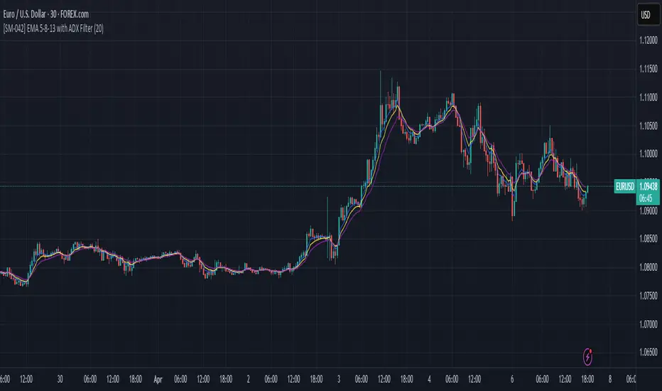
[SM-042] EMA 5-8-13 with ADX FilterWhat is the strategy?
The strategy combines three exponential moving averages (EMAs) — 5, 8, and 13 periods — with an optional ADX (Average Directional Index) filter. It is designed to enter long or short positions based on EMA crossovers and to exit positions when the price crosses a specific EMA. The ADX filter, if enabled, adds a condition that only allows trades when the ADX value is above a certain threshold, indicating trend strength.
Who is it for?
This strategy is for traders leveraging EMAs and trend strength indicators to make trade decisions. It can be used by anyone looking for a simple trend-following strategy, with the flexibility to adjust for trend strength using the ADX filter.
When is it used?
- **Long trades**: When the 5-period EMA crosses above the 8-period EMA, with an optional ADX condition (if enabled) that requires the ADX value to be above a specified threshold.
- **Short trades**: When the 5-period EMA crosses below the 8-period EMA, with the ADX filter again optional.
- **Exits**: The strategy exits a long position when the price falls below the 13-period EMA and exits a short position when the price rises above the 13-period EMA.
Where is it applied?
This strategy is applied on a chart with any asset on TradingView, with the EMAs and ADX plotted for visual reference. The strategy uses `strategy.entry` to open positions and `strategy.close` to close them based on the set conditions.
Why is it useful?
This strategy helps traders identify trending conditions and filter out potential false signals by using both EMAs (to capture short-term price movements) and the ADX (to confirm the strength of the trend). The ADX filter can be turned off if not desired, making the strategy flexible for both trending and range-bound markets.
How does it work?
- **EMA Crossover**: The strategy enters a long position when the 5-period EMA crosses above the 8-period EMA, and enters a short position when the 5-period EMA crosses below the 8-period EMA.
- **ADX Filter**: If enabled, the strategy checks whether the ADX value is above a set threshold (default is 20) before allowing a trade.
- **Exit Conditions**: Long positions are closed when the price falls below the 13-period EMA, and short positions are closed when the price rises above the 13-period EMA.
- **Plotting**: The strategy plots the three EMAs and the ADX value on the chart for visualization. It also displays a horizontal line at the ADX threshold.
This setup allows for clear decision-making based on the interaction between different time-frame EMAs and trend strength as indicated by ADX.
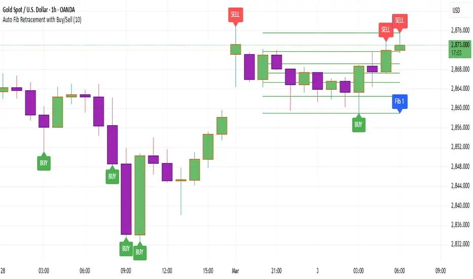
Auto Fib Retracement with Buy/SellKey Features of the Advanced Script:
Multi-Timeframe (MTF) Analysis:
We added an input for the higher timeframe (higher_tf), where the trend is checked on a higher timeframe to confirm the primary trend direction.
Complex Trend Detection:
The trend is determined not only by the current timeframe but also by the trend on the higher timeframe, giving a more comprehensive and reliable signal.
Dynamic Fibonacci Levels:
Fibonacci lines are plotted dynamically, extending them based on price movement, with the Fibonacci retracement drawn only when a trend is identified.
Background Color & Labels:
A background color is added to give a clear indication of the trend direction. Green for uptrend, red for downtrend. It makes it visually easier to understand the current market structure.
"Buy" or "Sell" labels are shown directly on the chart to mark possible entry points.
Strategy and Backtesting:
The script includes strategy commands (strategy.entry and strategy.exit), which allow for backtesting the strategy in TradingView.
Stop loss and take profit conditions are added (loss=100, profit=200), which can be adjusted according to your preferences.
Next Steps:
Test with different timeframes: Try changing the higher_tf to different timeframes (like "60" or "240") and see how it affects the trend detection.
Adjust Fibonacci settings: Modify how the Fibonacci levels are calculated or add more Fibonacci levels like 38.2%, 61.8%, etc.
Optimize Strategy Parameters: Fine-tune the entry/exit logic by adjusting stop loss, take profit, and other strategy parameters.
This should give you a robust foundation for creating advanced trend detection strategies
Strategy SuperTrend SDI WebhookThis Pine Script™ strategy is designed for automated trading in TradingView. It combines the SuperTrend indicator and Smoothed Directional Indicator (SDI) to generate buy and sell signals, with additional risk management features like stop loss, take profit, and trailing stop. The script also includes settings for leverage trading, equity-based position sizing, and webhook integration.
Key Features
1. Date-based Trade Execution
The strategy is active only between the start and end dates set by the user.
times ensures that trades occur only within this predefined time range.
2. Position Sizing and Leverage
Uses leverage trading to adjust position size dynamically based on initial equity.
The user can set leverage (leverage) and percentage of equity (usdprcnt).
The position size is calculated dynamically (initial_capital) based on account performance.
3. Take Profit, Stop Loss, and Trailing Stop
Take Profit (tp): Defines the target profit percentage.
Stop Loss (sl): Defines the maximum allowable loss per trade.
Trailing Stop (tr): Adjusts dynamically based on trade performance to lock in profits.
4. SuperTrend Indicator
SuperTrend (ta.supertrend) is used to determine the market trend.
If the price is above the SuperTrend line, it indicates an uptrend (bullish).
If the price is below the SuperTrend line, it signals a downtrend (bearish).
Plots visual indicators (green/red lines and circles) to show trend changes.
5. Smoothed Directional Indicator (SDI)
SDI helps to identify trend strength and momentum.
It calculates +DI (bullish strength) and -DI (bearish strength).
If +DI is higher than -DI, the market is considered bullish.
If -DI is higher than +DI, the market is considered bearish.
The background color changes based on the SDI signal.
6. Buy & Sell Conditions
Long Entry (Buy) Conditions:
SDI confirms an uptrend (+DI > -DI).
SuperTrend confirms an uptrend (price crosses above the SuperTrend line).
Short Entry (Sell) Conditions:
SDI confirms a downtrend (+DI < -DI).
SuperTrend confirms a downtrend (price crosses below the SuperTrend line).
Optionally, trades can be filtered using crossovers (occrs option).
7. Trade Execution and Exits
Market entries:
Long (strategy.entry("Long")) when conditions match.
Short (strategy.entry("Short")) when bearish conditions are met.
Trade exits:
Uses predefined take profit, stop loss, and trailing stop levels.
Positions are closed if the strategy is out of the valid time range.
Usage
Automated Trading Strategy:
Can be integrated with webhooks for automated execution on supported trading platforms.
Trend-Following Strategy:
Uses SuperTrend & SDI to identify trend direction and strength.
Risk-Managed Leverage Trading:
Supports position sizing, stop losses, and trailing stops.
Backtesting & Optimization:
Can be used for historical performance analysis before deploying live.
Conclusion
This strategy is suitable for traders who want to automate their trading using SuperTrend and SDI indicators. It incorporates risk management tools like stop loss, take profit, and trailing stop, making it adaptable for leverage trading. Traders can customize settings, conduct backtests, and integrate it with webhooks for real-time trade execution. 🚀
Important Note:
This script is provided for educational and template purposes and does not constitute financial advice. Traders and investors should conduct their research and analysis before making any trading decisions.

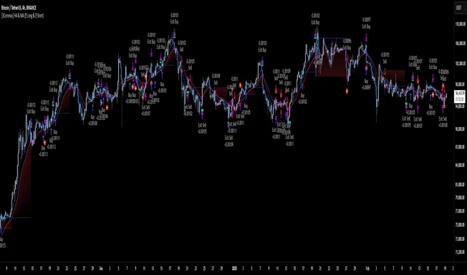
[3Commas] HA & MAHA & MA
🔷What it does: This tool is designed to test a trend-following strategy using Heikin Ashi candles and moving averages. It enters trades after pullbacks, aiming to let profits run once the risk-to-reward ratio reaches 1:1 while securing the position.
🔷Who is it for: It is ideal for traders looking to compare final results using fixed versus dynamic take profits by adjusting parameters and trade direction—a concept applicable to most trading strategies.
🔷How does it work: We use moving averages to define the market trend, then wait for opposite Heikin Ashi candles to form against it. Once these candles reverse in favor of the trend, we enter the trade, using the last swing created by the pullback as the stop loss. By applying the breakeven ratio, we protect the trade and let it run, using the slower moving average as a trailing stop.
A buy signal is generated when:
The previous candle is bearish (ha_bear ), indicating a pullback.
The fast moving average (ma1) is above the slow moving average (ma2), confirming an uptrend.
The current candle is bullish (ha_bull), showing trend continuation.
The Heikin Ashi close is above the fast moving average (ma1), reinforcing the bullish bias.
The real price close is above the open (close > open), ensuring bullish momentum in actual price data.
The signal is confirmed on the closed candle (barstate.isconfirmed) to avoid premature signals.
dir is undefined (na(dir)), preventing repeated signals in the same direction.
A sell signal is generated when:
The previous candle is bullish (ha_bull ), indicating a temporary upward move before a potential reversal.
The fast moving average (ma1) is below the slow moving average (ma2), confirming a downtrend.
The current candle is bearish (ha_bear), showing trend continuation to the downside.
The Heikin Ashi close is below the fast moving average (ma1), reinforcing bearish pressure.
The real price close is below the open (close < open), confirming bearish momentum in actual price data.
The signal is confirmed after the candle closes (barstate.isconfirmed), avoiding premature entries.
dir is undefined (na(dir)), preventing consecutive signals in the same direction.
In simple terms, this setup looks for trend continuation after a pullback, confirming entries with both Heikin Ashi and real price action, supported by moving average alignment to avoid false signals.
If the price reaches a 1:1 risk-to-reward ratio, the stop will be moved to the entry point. However, if the slow moving average surpasses this level, it will become the new exit point, acting as a trailing stop
🔷Why It’s Unique
Easily visualizes the benefits of using risk-to-reward ratios when trading instead of fixed percentages.
Provides a simple and straightforward approach to trading, embracing the "keep it simple" concept.
Offers clear visualization of DCA Bot entry and exit points based on user preferences.
Includes an option to review the message format before sending signals to bots, with compatibility for multi-pair and futures contract pairs.
🔷 Considerations Before Using the Indicator
⚠️Very important: The indicator must be used on charts with real price data, such as Japanese candlesticks, line charts, etc. Do not use it on Heikin Ashi charts, as this may lead to unrealistic results.
🔸Since this is a trend-following strategy, use it on timeframes above 4 hours, where market noise is reduced and trends are clearer. Also, carefully review the statistics before using it, focusing on pairs that tend to have long periods of well-defined trends.
🔸Disadvantages:
False Signals in Ranges: Consolidating markets can generate unreliable signals.
Lagging Indicator: Being based on moving averages, it may react late to sudden price movements.
🔸Advantages:
Trend Focused: Simplifies the identification of trending markets.
Noise Reduction: Uses Heikin Ashi candles to identify trend continuation after pullbacks.
Broad Applicability: Suitable for forex, crypto, stocks, and commodities.
🔸The strategy provides a systematic way to analyze markets but does not guarantee successful outcomes. Use it as an additional tool rather than relying solely on an automated system.
Trading results depend on various factors, including market conditions, trader discipline, and risk management. Past performance does not ensure future success, so always approach the market cautiously.
🔸Risk Management: Define stop-loss levels, position sizes, and profit targets before entering any trade. Be prepared for potential losses and ensure your approach aligns with your overall trading plan.
🔷 STRATEGY PROPERTIES
Symbol: BINANCE:BTCUSDT (Spot).
Timeframe: 4h.
Test Period: All historical data available.
Initial Capital: 10000 USDT.
Order Size per Trade: 1% of Capital, you can use a higher value e.g. 5%, be cautious that the Max Drawdown does not exceed 10%, as it would indicate a very risky trading approach.
Commission: Binance commission 0.1%, adjust according to the exchange being used, lower numbers will generate unrealistic results. By using low values e.g. 5%, it allows us to adapt over time and check the functioning of the strategy.
Slippage: 5 ticks, for pairs with low liquidity or very large orders, this number should be increased as the order may not be filled at the desired level.
Margin for Long and Short Positions: 100%.
Indicator Settings: Default Configuration.
MA1 Length: 9.
MA2 Length: 18.
MA Calculations: EMA.
Take Profit Ratio: Disable. Ratio 1:4.
Breakeven Ratio: Enable, Ratio 1:1.
Strategy: Long & Short.
🔷 STRATEGY RESULTS
⚠️Remember, past results do not guarantee future performance.
Net Profit: +324.88 USDT (+3.25%).
Max Drawdown: -81.18 USDT (-0.78%).
Total Closed Trades: 672.
Percent Profitable: 35.57%.
Profit Factor: 1.347.
Average Trade: +0.48 USDT (+0.48%).
Average # Bars in Trades: 13.
🔷 HOW TO USE
🔸 Adjust Settings:
The default values—MA1 (9) and MA2 (18) with EMA calculation—generally work well. However, you can increase these values, such as 20 and 40, to better identify stronger trends.
🔸 Choose a Symbol that Typically Trends:
Select an asset that tends to form clear trends. Keep in mind that the Strategy Tester results may show poor performance for certain assets, making them less suitable for sending signals to bots.
🔸 Experiment with Ratios:
Test different take profit and breakeven ratios to compare various scenarios—especially to observe how the strategy performs when only the trade is protected.
🔸This is an example of how protecting the trade works: once the price moves in favor of the position with a 1:1 risk-to-reward ratio, the stop loss is moved to the entry price. If the Slow MA surpasses this level, it will act as a trailing stop, aiming to follow the trend and maximize potential gains.
🔸In contrast, in this example, for the same trade, if we set a take profit at a 1:3 risk-to-reward ratio—which is generally considered a good risk-reward relationship—we can see how a significant portion of the upward move is left on the table.
🔸Results Review:
It is important to check the Max Drawdown. This value should ideally not exceed 10% of your capital. Consider adjusting the trade size to ensure this threshold is not surpassed.
Remember to include the correct values for commission and slippage according to the symbol and exchange where you are conducting the tests. Otherwise, the results will not be realistic.
If you are satisfied with the results, you may consider automating your trades. However, it is strongly recommended to use a small amount of capital or a demo account to test proper execution before committing real funds.
🔸Create alerts to trigger the DCA Bot:
Verify Messages: Ensure the message matches the one specified by the DCA Bot.
Multi-Pair Configuration: For multi-pair setups, enable the option to add the symbol in the correct format.
Signal Settings: Enable whether you want to receive long or short signals (Entry | TP | SL), copy and paste the the messages for the DCA Bots configured.
Alert Setup:
When creating an alert, set the condition to the indicator and choose "alert() function call only.
Enter any desired Alert Name.
Open the Notifications tab, enable Webhook URL, and paste the Webhook URL.
For more details, refer to the section: "How to use TradingView Custom Signals".
Finalize Alerts: Click Create, you're done! Alerts will now be sent automatically in the correct format.
🔷 INDICATOR SETTINGS
MA 1: Fast MA Length
MA 2: Slow MA Length
MA Calc: MA's Calculations (SMA,EMA, RMA,WMA)
TP Ratio: This is the take profit ratio relative to the stop loss, where the trade will be closed in profit.
BE Ratio: This is the breakeven ratio relative to the stop loss, where the stop loss will be updated to breakeven or if the MA2 is greater than this level.
Strategy: Order Type direction in which trades are executed.
Use Custom Test Period: When enabled signals only works in the selected time window. If disabled it will use all historical data available on the chart.
Test Start and End: Once the Custom Test Period is enabled, here you select the start and end date that you want to analyze.
Check Messages: Enable the table to review the messages to be sent to the bot.
Entry | TP | SL: Enable this options to send Buy Entry, Take Profit (TP), and Stop Loss (SL) signals.
Deal Entry and Deal Exit : Copy and paste the message for the deal start signal and close order at Market Price of the DCA Bot. This is the message that will be sent with the alert to the Bot, you must verify that it is the same as the bot so that it can process properly so that it executes and starts the trade.
DCA Bot Multi-Pair: You must activate it if you want to use the signals in a DCA Bot Multi-pair in the text box you must enter (using the correct format) the symbol in which you are creating the alert, you can check the format of each symbol when you create the bot.
👨🏻💻💭 We hope this tool helps enhance your trading. Your feedback is invaluable, so feel free to share any suggestions for improvements or new features you'd like to see implemented.
__
The information and publications within the 3Commas TradingView account are not meant to be and do not constitute financial, investment, trading, or other types of advice or recommendations supplied or endorsed by 3Commas and any of the parties acting on behalf of 3Commas, including its employees, contractors, ambassadors, etc.
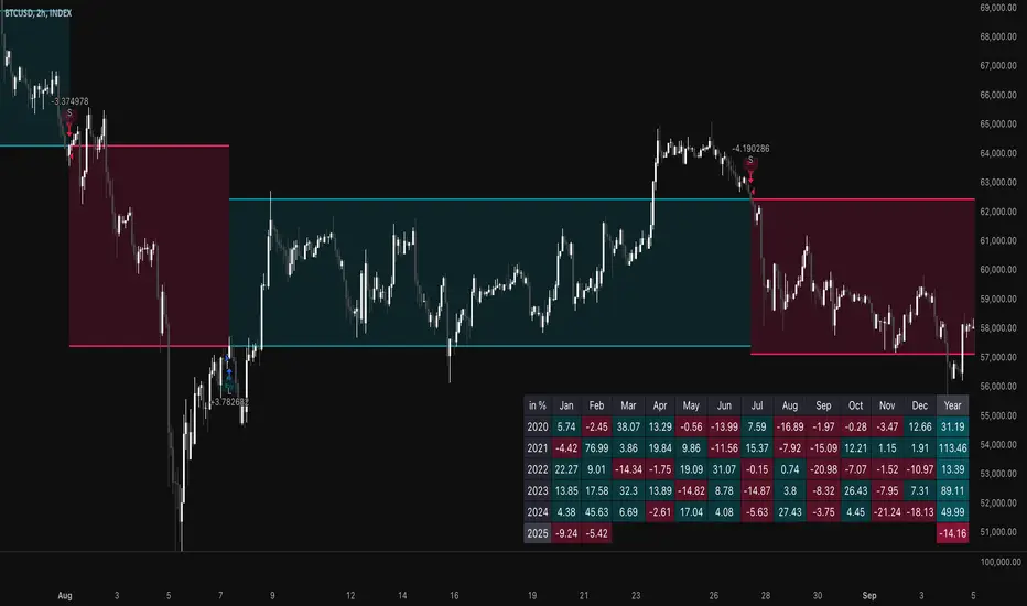
TSI Long/Short for BTC 2HThe TSI Long/Short for BTC 2H strategy is an advanced trend-following system designed specifically for trading Bitcoin (BTC) on a 2-hour timeframe. It leverages the True Strength Index (TSI) to identify momentum shifts and executes both long and short trades in response to dynamic market conditions.
Unlike traditional moving average-based strategies, this script uses a double-smoothed momentum calculation, enhancing signal accuracy and reducing noise. It incorporates automated position sizing, customizable leverage, and real-time performance tracking, ensuring a structured and adaptable trading approach.
🔹 What Makes This Strategy Unique?
Unlike simple crossover strategies or generic trend-following approaches, this system utilizes a customized True Strength Index (TSI) methodology that dynamically adjusts to market conditions.
🔸 True Strength Index (TSI) Filtering – The script refines the TSI by applying double exponential smoothing, filtering out weak signals and capturing high-confidence momentum shifts.
🔸 Adaptive Entry & Exit Logic – Instead of fixed thresholds, it compares the TSI value against a dynamically determined high/low range from the past 100 bars to confirm trade signals.
🔸 Leverage & Risk Optimization – Position sizing is dynamically adjusted based on account equity and leverage settings, ensuring controlled risk exposure.
🔸 Performance Monitoring System – A built-in performance tracking table allows traders to evaluate monthly and yearly results directly on the chart.
📊 Core Strategy Components
1️⃣ Momentum-Based Trade Execution
The strategy generates long and short trade signals based on the following conditions:
✅ Long Entry Condition – A buy signal is triggered when the TSI crosses above its 100-bar highest value (previously set), confirming bullish momentum.
✅ Short Entry Condition – A sell signal is generated when the TSI crosses below its 100-bar lowest value (previously set), indicating bearish pressure.
Each trade execution is fully automated, reducing emotional decision-making and improving trading discipline.
2️⃣ Position Sizing & Leverage Control
Risk management is a key focus of this strategy:
🔹 Dynamic Position Sizing – The script calculates position size based on:
Account Equity – Ensuring trade sizes adjust dynamically with capital fluctuations.
Leverage Multiplier – Allows traders to customize risk exposure via an adjustable leverage setting.
🔹 No Fixed Stop-Loss – The strategy relies on reversals to exit trades, meaning each position is closed when the opposite signal appears.
This design ensures maximum capital efficiency while adapting to market conditions in real time.
3️⃣ Performance Visualization & Tracking
Understanding historical performance is crucial for refining strategies. The script includes:
📌 Real-Time Trade Markers – Buy and sell signals are visually displayed on the chart for easy reference.
📌 Performance Metrics Table – Tracks monthly and yearly returns in percentage form, helping traders assess profitability over time.
📌 Trade History Visualization – Completed trades are displayed with color-coded boxes (green for long trades, red for short trades), visually representing profit/loss dynamics.
📢 Why Use This Strategy?
✔ Advanced Momentum Detection – Uses a double-smoothed TSI for more accurate trend signals.
✔ Fully Automated Trading – Removes emotional bias and enforces discipline.
✔ Customizable Risk Management – Adjust leverage and position sizing to suit your risk profile.
✔ Comprehensive Performance Tracking – Integrated reporting system provides clear insights into past trades.
This strategy is ideal for Bitcoin traders looking for a structured, high-probability system that adapts to both bullish and bearish trends on the 2-hour timeframe.
📌 How to Use: Simply add the script to your 2H BTC chart, configure your leverage settings, and let the system handle trade execution and tracking! 🚀
00 Averaging Down Backtest Strategy by RPAlawyer v21FOR EDUCATIONAL PURPOSES ONLY! THE CODE IS NOT YET FULLY DEVELOPED, BUT IT CAN PROVIDE INTERESTING DATA AND INSIGHTS IN ITS CURRENT STATE.
This strategy is an 'averaging down' backtester strategy. The goal of averaging/doubling down is to buy more of an asset at a lower price to reduce your average entry price.
This backtester code proves why you shouldn't do averaging down, but the code can be developed (and will be developed) further, and there might be settings even in its current form that prove that averaging down can be done effectively.
Different averaging down strategies exist:
- Linear/Fixed Amount: buy $1000 every time price drops 5%
- Grid Trading: Placing orders at price levels, often with increasing size, like $1000 at -5%, $2000 at -10%
- Martingale: doubling the position size with each new entry
- Reverse Martingale: decreasing position size as price falls: $4000, then $2000, then $1000
- Percentage-Based: position size based on % of remaining capital, like 10% of available funds at each level
- Dynamic/Adaptive: larger entries during high volatility, smaller during low
- Logarithmic: position sizes increase logarithmically as price drops
Unlike the above average costing strategies, it applies averaging down (I use DCA as a synonym) at a very strong trend reversal. So not at a certain predetermined percentage negative PNL % but at a trend reversal signaled by an indicator - hence it most closely resembles a dynamically moving grid DCA strategy.
Both entering the trade and averaging down assume a strong trend. The signals for trend detection are provided by an indicator that I published under the name '00 Parabolic SAR Trend Following Signals by RPAlawyer', but any indicator that generates numeric signals of 1 and -1 for buy and sell signals can be used.
The indicator must be connected to the strategy: in the strategy settings under 'External Source' you need to select '00 Parabolic SAR Trend Following Signals by RPAlawyer: Connector'. From this point, the strategy detects when the indicator generates buy and sell signals.
The strategy considers a strong trend when a buy signal appears above a very conservative ATR band, or a sell signal below the ATR band. The conservative ATR is chosen to filter ranging markets. This very conservative ATR setting has a default multiplier of 8 and length of 40. The multiplier can be increased up to 10, but there will be very few buy and sell signals at that level and DCA requirements will be very high. Trade entry and DCA occur at these strong trends. In the settings, the 'ATR Filter' setting determines the entry condition (e.g., ATR Filter multiplier of 9), and the 'DCA ATR' determines when DCA will happen (e.g., DCA ATR multiplier of 6).
The DCA levels and DCA amounts are determined as follows:
The first DCA occurs below the DCA Base Deviation% level (see settings, default 3%) which acts as a threshold. The thick green line indicates the long position avg price, and the thin red line below the green line indicates the 3% DCA threshold for long positions. The thick red line indicates the short position avg price, and the thin red line above the thick red line indicates the short position 3% DCA threshold. DCA size multiplier defines the DCA amount invested.
If the loss exceeds 3% AND a buy signal arrives below the lower ATR band for longs, or a sell signal arrives above the upper ATR band for shorts, then the first DCA will be executed. So the first DCA won't happen at 3%, rather 3% is a threshold where the additional condition is that the price must close above or below the ATR band (let's say the first DCA occured at 8%) – this is why the code resembles a dynamic grid strategy, where the grid moves such that alongside the first 3% threshold, a strong trend must also appear for DCA. At this point, the thick green/red line moves because the avg price is modified as a result of the DCA, and the thin red line indicating the next DCA level also moves. The next DCA level is determined by the first DCA level, meaning modified avg price plus an additional +8% + (3% * the Step Scale Multiplier in the settings). This next DCA level will be indicated by the modified thin red line, and the price must break through this level and again break through the ATR band for the second DCA to occur.
Since all this wasn't complicated enough, and I was always obsessed by the idea that when we're sitting in an underwater position for days, doing DCA and waiting for the price to correct, we can actually enter a short position on the other side, on which we can realize profit (if the broker allows taking hedge positions, Binance allows this in Europe).
This opposite position in this strategy can open from the point AFTER THE FIRST DCA OF THE BASE POSITION OCCURS. This base position first DCA actually indicates that the price has already moved against us significantly so time to earn some money on the other side. Breaking through the ATR band is also a condition for entry here, so the hedge position entry is not automatic, and the condition for further DCA is breaking through the DCA Base Deviation (default 3%) and breaking through the ATR band. So for the 'hedge' or rather opposite position, the entry and further DCA conditions are the same as for the base position. The hedge position avg price is indicated by a thick black line and the Next Hedge DCA Level is indicated by a thin black line.
The TPs are indicated by green labels for base positions and red labels for hedge positions.
No SL built into the strategy at this point but you are free to do your coding.
Summary data can be found in the upper right corner.
The fantastic trend reversal indicator Machine learning: Lorentzian Classification by jdehorty can be used as an external indicator, choose 'backtest stream' for the external source. The ATR Band multiplicators need to be reduced to 5-6 when using Lorentz.
The code can be further developed in several aspects, and as I write this, I already have a few ideas 😊

Z-Strike RecoveryThis strategy utilizes the Z-Score of daily changes in the VIX (Volatility Index) to identify moments of extreme market panic and initiate long entries. Scientific research highlights that extreme volatility levels often signal oversold markets, providing opportunities for mean-reversion strategies.
How the Strategy Works
Calculation of Daily VIX Changes:
The difference between today’s and yesterday’s VIX closing prices is calculated.
Z-Score Calculation:
The Z-Score quantifies how far the current change deviates from the mean (average), expressed in standard deviations:
Z-Score=(Daily VIX Change)−MeanStandard Deviation
Z-Score=Standard Deviation(Daily VIX Change)−Mean
The mean and standard deviation are computed over a rolling period of 16 days (default).
Entry Condition:
A long entry is triggered when the Z-Score exceeds a threshold of 1.3 (adjustable).
A high positive Z-Score indicates a strong overreaction in the market (panic).
Exit Condition:
The position is closed after 10 periods (days), regardless of market behavior.
Visualizations:
The Z-Score is plotted to make extreme values visible.
Horizontal threshold lines mark entry signals.
Bars with entry signals are highlighted with a blue background.
This strategy is particularly suitable for mean-reverting markets, such as the S&P 500.
Scientific Background
Volatility and Market Behavior:
Studies like Whaley (2000) demonstrate that the VIX, known as the "fear gauge," is highly correlated with market panic phases. A spike in the VIX is often interpreted as an oversold signal due to excessive hedging by investors.
Source: Whaley, R. E. (2000). The investor fear gauge. Journal of Portfolio Management, 26(3), 12-17.
Z-Score in Financial Strategies:
The Z-Score is a proven method for detecting statistical outliers and is widely used in mean-reversion strategies.
Source: Chan, E. (2009). Quantitative Trading. Wiley Finance.
Mean-Reversion Approach:
The strategy builds on the mean-reversion principle, which assumes that extreme market movements tend to revert to the mean over time.
Source: Jegadeesh, N., & Titman, S. (1993). Returns to Buying Winners and Selling Losers: Implications for Stock Market Efficiency. Journal of Finance, 48(1), 65-91.

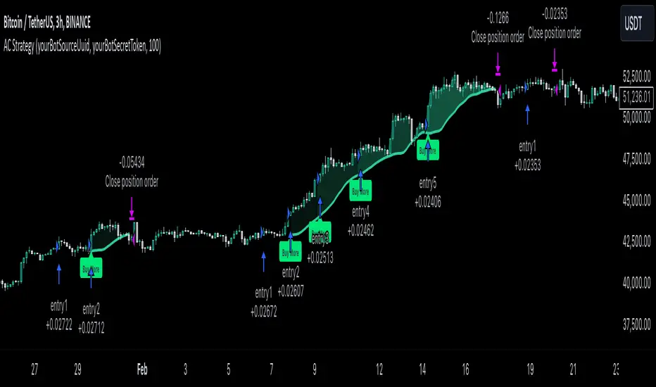
MultiLayer Acceleration/Deceleration Strategy [Skyrexio]Overview
MultiLayer Acceleration/Deceleration Strategy leverages the combination of Acceleration/Deceleration Indicator(AC), Williams Alligator, Williams Fractals and Exponential Moving Average (EMA) to obtain the high probability long setups. Moreover, strategy uses multi trades system, adding funds to long position if it considered that current trend has likely became stronger. Acceleration/Deceleration Indicator is used for creating signals, while Alligator and Fractal are used in conjunction as an approximation of short-term trend to filter them. At the same time EMA (default EMA's period = 100) is used as high probability long-term trend filter to open long trades only if it considers current price action as an uptrend. More information in "Methodology" and "Justification of Methodology" paragraphs. The strategy opens only long trades.
Unique Features
No fixed stop-loss and take profit: Instead of fixed stop-loss level strategy utilizes technical condition obtained by Fractals and Alligator to identify when current uptrend is likely to be over (more information in "Methodology" and "Justification of Methodology" paragraphs)
Configurable Trading Periods: Users can tailor the strategy to specific market windows, adapting to different market conditions.
Multilayer trades opening system: strategy uses only 10% of capital in every trade and open up to 5 trades at the same time if script consider current trend as strong one.
Short and long term trend trade filters: strategy uses EMA as high probability long-term trend filter and Alligator and Fractal combination as a short-term one.
Methodology
The strategy opens long trade when the following price met the conditions:
1. Price closed above EMA (by default, period = 100). Crossover is not obligatory.
2. Combination of Alligator and Williams Fractals shall consider current trend as an upward (all details in "Justification of Methodology" paragraph)
3. Acceleration/Deceleration shall create one of two types of long signals (all details in "Justification of Methodology" paragraph). Buy stop order is placed one tick above the candle's high of last created long signal.
4. If price reaches the order price, long position is opened with 10% of capital.
5. If currently we have opened position and price creates and hit the order price of another one long signal, another one long position will be added to the previous with another one 10% of capital. Strategy allows to open up to 5 long trades simultaneously.
6. If combination of Alligator and Williams Fractals shall consider current trend has been changed from up to downtrend, all long trades will be closed, no matter how many trades has been opened.
Script also has additional visuals. If second long trade has been opened simultaneously the Alligator's teeth line is plotted with the green color. Also for every trade in a row from 2 to 5 the label "Buy More" is also plotted just below the teeth line. With every next simultaneously opened trade the green color of the space between teeth and price became less transparent.
Strategy settings
In the inputs window user can setup strategy setting: EMA Length (by default = 100, period of EMA, used for long-term trend filtering EMA calculation). User can choose the optimal parameters during backtesting on certain price chart.
Justification of Methodology
Let's explore the key concepts of this strategy and understand how they work together. We'll begin with the simplest: the EMA.
The Exponential Moving Average (EMA) is a type of moving average that assigns greater weight to recent price data, making it more responsive to current market changes compared to the Simple Moving Average (SMA). This tool is widely used in technical analysis to identify trends and generate buy or sell signals. The EMA is calculated as follows:
1.Calculate the Smoothing Multiplier:
Multiplier = 2 / (n + 1), Where n is the number of periods.
2. EMA Calculation
EMA = (Current Price) × Multiplier + (Previous EMA) × (1 − Multiplier)
In this strategy, the EMA acts as a long-term trend filter. For instance, long trades are considered only when the price closes above the EMA (default: 100-period). This increases the likelihood of entering trades aligned with the prevailing trend.
Next, let’s discuss the short-term trend filter, which combines the Williams Alligator and Williams Fractals. Williams Alligator
Developed by Bill Williams, the Alligator is a technical indicator that identifies trends and potential market reversals. It consists of three smoothed moving averages:
Jaw (Blue Line): The slowest of the three, based on a 13-period smoothed moving average shifted 8 bars ahead.
Teeth (Red Line): The medium-speed line, derived from an 8-period smoothed moving average shifted 5 bars forward.
Lips (Green Line): The fastest line, calculated using a 5-period smoothed moving average shifted 3 bars forward.
When the lines diverge and align in order, the "Alligator" is "awake," signaling a strong trend. When the lines overlap or intertwine, the "Alligator" is "asleep," indicating a range-bound or sideways market. This indicator helps traders determine when to enter or avoid trades.
Fractals, another tool by Bill Williams, help identify potential reversal points on a price chart. A fractal forms over at least five consecutive bars, with the middle bar showing either:
Up Fractal: Occurs when the middle bar has a higher high than the two preceding and two following bars, suggesting a potential downward reversal.
Down Fractal: Happens when the middle bar shows a lower low than the surrounding two bars, hinting at a possible upward reversal.
Traders often use fractals alongside other indicators to confirm trends or reversals, enhancing decision-making accuracy.
How do these tools work together in this strategy? Let’s consider an example of an uptrend.
When the price breaks above an up fractal, it signals a potential bullish trend. This occurs because the up fractal represents a shift in market behavior, where a temporary high was formed due to selling pressure. If the price revisits this level and breaks through, it suggests the market sentiment has turned bullish.
The breakout must occur above the Alligator’s teeth line to confirm the trend. A breakout below the teeth is considered invalid, and the downtrend might still persist. Conversely, in a downtrend, the same logic applies with down fractals.
In this strategy if the most recent up fractal breakout occurs above the Alligator's teeth and follows the last down fractal breakout below the teeth, the algorithm identifies an uptrend. Long trades can be opened during this phase if a signal aligns. If the price breaks a down fractal below the teeth line during an uptrend, the strategy assumes the uptrend has ended and closes all open long trades.
By combining the EMA as a long-term trend filter with the Alligator and fractals as short-term filters, this approach increases the likelihood of opening profitable trades while staying aligned with market dynamics.
Now let's talk about Acceleration/Deceleration signals. AC indicator is calculated using the Awesome Oscillator, so let's first of all briefly explain what is Awesome Oscillator and how it can be calculated. The Awesome Oscillator (AO), developed by Bill Williams, is a momentum indicator designed to measure market momentum by contrasting recent price movements with a longer-term historical perspective. It helps traders detect potential trend reversals and assess the strength of ongoing trends.
The formula for AO is as follows:
AO = SMA5(Median Price) − SMA34(Median Price)
where:
Median Price = (High + Low) / 2
SMA5 = 5-period Simple Moving Average of the Median Price
SMA 34 = 34-period Simple Moving Average of the Median Price
The Acceleration/Deceleration (AC) Indicator, introduced by Bill Williams, measures the rate of change in market momentum. It highlights shifts in the driving force of price movements and helps traders spot early signs of trend changes. The AC Indicator is particularly useful for identifying whether the current momentum is accelerating or decelerating, which can indicate potential reversals or continuations. For AC calculation we shall use the AO calculated above is the following formula:
AC = AO − SMA5(AO), where SMA5(AO)is the 5-period Simple Moving Average of the Awesome Oscillator
When the AC is above the zero line and rising, it suggests accelerating upward momentum.
When the AC is below the zero line and falling, it indicates accelerating downward momentum.
When the AC is below zero line and rising it suggests the decelerating the downtrend momentum. When AC is above the zero line and falling, it suggests the decelerating the uptrend momentum.
Now we can explain which AC signal types are used in this strategy. The first type of long signal is when AC value is below zero line. In this cases we need to see three rising bars on the histogram in a row after the falling one. The second type of signals occurs above the zero line. There we need only two rising AC bars in a row after the falling one to create the signal. The signal bar is the last green bar in this sequence. The strategy places the buy stop order one tick above the candle's high, which corresponds to the signal bar on AC indicator.
After that we can have the following scenarios:
Price hit the order on the next candle in this case strategy opened long with this price.
Price doesn't hit the order price, the next candle set lower high. If current AC bar is increasing buy stop order changes by the script to the high of this new bar plus one tick. This procedure repeats until price finally hit buy order or current AC bar become decreasing. In the second case buy order cancelled and strategy wait for the next AC signal.
If long trades are initiated, the strategy continues utilizing subsequent signals until the total number of trades reaches a maximum of 5. All open trades are closed when the trend shifts to a downtrend, as determined by the combination of the Alligator and Fractals described earlier.
Why we use AC signals? If currently strategy algorithm considers the high probability of the short-term uptrend with the Alligator and Fractals combination pointed out above and the long-term trend is also suggested by the EMA filter as bullish. Rising AC bars after period of falling AC bars indicates the high probability of local pull back end and there is a high chance to open long trade in the direction of the most likely main uptrend. The numbers of rising bars are different for the different AC values (below or above zero line). This is needed because if AC below zero line the local downtrend is likely to be stronger and needs more rising bars to confirm that it has been changed than if AC is above zero.
Why strategy use only 10% per signal? Sometimes we can see the false signals which appears on sideways. Not risking that much script use only 10% per signal. If the first long trade has been open and price continue going up and our trend approximation by Alligator and Fractals is uptrend, strategy add another one 10% of capital to every next AC signal while number of active trades no more than 5. This capital allocation allows to take part in long trades when current uptrend is likely to be strong and use only 10% of capital when there is a high probability of sideways.
Backtest Results
Operating window: Date range of backtests is 2023.01.01 - 2024.11.01. It is chosen to let the strategy to close all opened positions.
Commission and Slippage: Includes a standard Binance commission of 0.1% and accounts for possible slippage over 5 ticks.
Initial capital: 10000 USDT
Percent of capital used in every trade: 10%
Maximum Single Position Loss: -5.15%
Maximum Single Profit: +24.57%
Net Profit: +2108.85 USDT (+21.09%)
Total Trades: 111 (36.94% win rate)
Profit Factor: 2.391
Maximum Accumulated Loss: 367.61 USDT (-2.97%)
Average Profit per Trade: 19.00 USDT (+1.78%)
Average Trade Duration: 75 hours
How to Use
Add the script to favorites for easy access.
Apply to the desired timeframe and chart (optimal performance observed on 3h BTC/USDT).
Configure settings using the dropdown choice list in the built-in menu.
Set up alerts to automate strategy positions through web hook with the text: {{strategy.order.alert_message}}
Disclaimer:
Educational and informational tool reflecting Skyrex commitment to informed trading. Past performance does not guarantee future results. Test strategies in a simulated environment before live implementation
These results are obtained with realistic parameters representing trading conditions observed at major exchanges such as Binance and with realistic trading portfolio usage parameters.
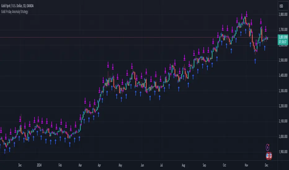
Gold Friday Anomaly StrategyThis script implements the " Gold Friday Anomaly Strategy ," a well-known historical trading strategy that leverages the gold market's behavior from Thursday evening to Friday close. It is a backtesting-focused strategy designed to assess the historical performance of this pattern. Traders use this anomaly as it captures a recurring market tendency observed over the years.
What It Does:
Entry Condition: The strategy enters a long position at the beginning of the Friday trading session (Thursday evening close) within the defined backtesting period.
Exit Condition: Friday evening close.
Backtesting Controls: Allows users to set custom backtesting periods to evaluate strategy performance over specific date ranges.
Key Features:
Custom Backtest Periods: Easily configurable inputs to set the start and end date of the backtesting range.
Fixed Slippage and Commission Settings: Ensures realistic simulation of trading conditions.
Process Orders on Close: Backtesting is optimized by processing orders at the bar's close.
Important Notes:
Backtesting Only: This script is intended purely for backtesting purposes. Past performance is not indicative of future results.
Live Trading Recommendations: For live trading, it is highly recommended to use limit orders instead of market orders, especially during evening sessions, as market order slippage can be significant.
Default Settings:
Entry size: 10% of equity per trade.
Slippage: 1 tick.
Commission: 0.05% per trade.
MultiLayer Awesome Oscillator Saucer Strategy [Skyrexio]Overview
MultiLayer Awesome Oscillator Saucer Strategy leverages the combination of Awesome Oscillator (AO), Williams Alligator, Williams Fractals and Exponential Moving Average (EMA) to obtain the high probability long setups. Moreover, strategy uses multi trades system, adding funds to long position if it considered that current trend has likely became stronger. Awesome Oscillator is used for creating signals, while Alligator and Fractal are used in conjunction as an approximation of short-term trend to filter them. At the same time EMA (default EMA's period = 100) is used as high probability long-term trend filter to open long trades only if it considers current price action as an uptrend. More information in "Methodology" and "Justification of Methodology" paragraphs. The strategy opens only long trades.
Unique Features
No fixed stop-loss and take profit: Instead of fixed stop-loss level strategy utilizes technical condition obtained by Fractals and Alligator to identify when current uptrend is likely to be over (more information in "Methodology" and "Justification of Methodology" paragraphs)
Configurable Trading Periods: Users can tailor the strategy to specific market windows, adapting to different market conditions.
Multilayer trades opening system: strategy uses only 10% of capital in every trade and open up to 5 trades at the same time if script consider current trend as strong one.
Short and long term trend trade filters: strategy uses EMA as high probability long-term trend filter and Alligator and Fractal combination as a short-term one.
Methodology
The strategy opens long trade when the following price met the conditions:
1. Price closed above EMA (by default, period = 100). Crossover is not obligatory.
2. Combination of Alligator and Williams Fractals shall consider current trend as an upward (all details in "Justification of Methodology" paragraph)
3. Awesome Oscillator shall create the "Saucer" long signal (all details in "Justification of Methodology" paragraph). Buy stop order is placed one tick above the candle's high of last created "Saucer signal".
4. If price reaches the order price, long position is opened with 10% of capital.
5. If currently we have opened position and price creates and hit the order price of another one "Saucer" signal another one long position will be added to the previous with another one 10% of capital. Strategy allows to open up to 5 long trades simultaneously.
6. If combination of Alligator and Williams Fractals shall consider current trend has been changed from up to downtrend, all long trades will be closed, no matter how many trades has been opened.
Script also has additional visuals. If second long trade has been opened simultaneously the Alligator's teeth line is plotted with the green color. Also for every trade in a row from 2 to 5 the label "Buy More" is also plotted just below the teeth line. With every next simultaneously opened trade the green color of the space between teeth and price became less transparent.
Strategy settings
In the inputs window user can setup strategy setting: EMA Length (by default = 100, period of EMA, used for long-term trend filtering EMA calculation). User can choose the optimal parameters during backtesting on certain price chart.
Justification of Methodology
Let's go through all concepts used in this strategy to understand how they works together. Let's start from the easies one, the EMA. Let's briefly explain what is EMA. The Exponential Moving Average (EMA) is a type of moving average that gives more weight to recent prices, making it more responsive to current price changes compared to the Simple Moving Average (SMA). It is commonly used in technical analysis to identify trends and generate buy or sell signals. It can be calculated with the following steps:
1.Calculate the Smoothing Multiplier:
Multiplier = 2 / (n + 1), Where n is the number of periods.
2. EMA Calculation
EMA = (Current Price) × Multiplier + (Previous EMA) × (1 − Multiplier)
In this strategy uses EMA an initial long term trend filter. It allows to open long trades only if price close above EMA (by default 50 period). It increases the probability of taking long trades only in the direction of the trend.
Let's go to the next, short-term trend filter which consists of Alligator and Fractals. Let's briefly explain what do these indicators means. The Williams Alligator, developed by Bill Williams, is a technical indicator designed to spot trends and potential market reversals. It uses three smoothed moving averages, referred to as the jaw, teeth, and lips:
Jaw (Blue Line): The slowest of the three, based on a 13-period smoothed moving average shifted 8 bars ahead.
Teeth (Red Line): The medium-speed line, derived from an 8-period smoothed moving average shifted 5 bars forward.
Lips (Green Line): The fastest line, calculated using a 5-period smoothed moving average shifted 3 bars forward.
When these lines diverge and are properly aligned, the "alligator" is considered "awake," signaling a strong trend. Conversely, when the lines overlap or intertwine, the "alligator" is "asleep," indicating a range-bound or sideways market. This indicator assists traders in identifying when to act on or avoid trades.
The Williams Fractals, another tool introduced by Bill Williams, are used to pinpoint potential reversal points on a price chart. A fractal forms when there are at least five consecutive bars, with the middle bar displaying the highest high (for an up fractal) or the lowest low (for a down fractal), relative to the two bars on either side.
Key Points:
Up Fractal: Occurs when the middle bar has a higher high than the two preceding and two following bars, suggesting a potential downward reversal.
Down Fractal: Happens when the middle bar shows a lower low than the surrounding two bars, hinting at a possible upward reversal.
Traders often combine fractals with other indicators to confirm trends or reversals, improving the accuracy of trading decisions.
How we use their combination in this strategy? Let’s consider an uptrend example. A breakout above an up fractal can be interpreted as a bullish signal, indicating a high likelihood that an uptrend is beginning. Here's the reasoning: an up fractal represents a potential shift in market behavior. When the fractal forms, it reflects a pullback caused by traders selling, creating a temporary high. However, if the price manages to return to that fractal’s high and break through it, it suggests the market has "changed its mind" and a bullish trend is likely emerging.
The moment of the breakout marks the potential transition to an uptrend. It’s crucial to note that this breakout must occur above the Alligator's teeth line. If it happens below, the breakout isn’t valid, and the downtrend may still persist. The same logic applies inversely for down fractals in a downtrend scenario.
So, if last up fractal breakout was higher, than Alligator's teeth and it happened after last down fractal breakdown below teeth, algorithm considered current trend as an uptrend. During this uptrend long trades can be opened if signal was flashed. If during the uptrend price breaks down the down fractal below teeth line, strategy considered that uptrend is finished with the high probability and strategy closes all current long trades. This combination is used as a short term trend filter increasing the probability of opening profitable long trades in addition to EMA filter, described above.
Now let's talk about Awesome Oscillator's "Sauser" signals. Briefly explain what is the Awesome Oscillator. The Awesome Oscillator (AO), created by Bill Williams, is a momentum-based indicator that evaluates market momentum by comparing recent price activity to a broader historical context. It assists traders in identifying potential trend reversals and gauging trend strength.
AO = SMA5(Median Price) − SMA34(Median Price)
where:
Median Price = (High + Low) / 2
SMA5 = 5-period Simple Moving Average of the Median Price
SMA 34 = 34-period Simple Moving Average of the Median Price
Now we know what is AO, but what is the "Saucer" signal? This concept was introduced by Bill Williams, let's briefly explain it and how it's used by this strategy. Initially, this type of signal is a combination of the following AO bars: we need 3 bars in a row, the first one shall be higher than the second, the third bar also shall be higher, than second. All three bars shall be above the zero line of AO. The price bar, which corresponds to third "saucer's" bar is our signal bar. Strategy places buy stop order one tick above the price bar which corresponds to signal bar.
After that we can have the following scenarios.
Price hit the order on the next candle in this case strategy opened long with this price.
Price doesn't hit the order price, the next candle set lower low. If current AO bar is increasing buy stop order changes by the script to the high of this new bar plus one tick. This procedure repeats until price finally hit buy order or current AO bar become decreasing. In the second case buy order cancelled and strategy wait for the next "Saucer" signal.
If long trades has been opened strategy use all the next signals until number of trades doesn't exceed 5. All trades are closed when the trend changes to downtrend according to combination of Alligator and Fractals described above.
Why we use "Saucer" signals? If AO above the zero line there is a high probability that price now is in uptrend if we take into account our two trend filters. When we see the decreasing bars on AO and it's above zero it's likely can be considered as a pullback on the uptrend. When we see the stop of AO decreasing and the first increasing bar has been printed there is a high probability that this local pull back is finished and strategy open long trade in the likely direction of a main trend.
Why strategy use only 10% per signal? Sometimes we can see the false signals which appears on sideways. Not risking that much script use only 10% per signal. If the first long trade has been open and price continue going up and our trend approximation by Alligator and Fractals is uptrend, strategy add another one 10% of capital to every next saucer signal while number of active trades no more than 5. This capital allocation allows to take part in long trades when current uptrend is likely to be strong and use only 10% of capital when there is a high probability of sideways.
Backtest Results
Operating window: Date range of backtests is 2023.01.01 - 2024.11.25. It is chosen to let the strategy to close all opened positions.
Commission and Slippage: Includes a standard Binance commission of 0.1% and accounts for possible slippage over 5 ticks.
Initial capital: 10000 USDT
Percent of capital used in every trade: 10%
Maximum Single Position Loss: -5.10%
Maximum Single Profit: +22.80%
Net Profit: +2838.58 USDT (+28.39%)
Total Trades: 107 (42.99% win rate)
Profit Factor: 3.364
Maximum Accumulated Loss: 373.43 USDT (-2.98%)
Average Profit per Trade: 26.53 USDT (+2.40%)
Average Trade Duration: 78 hours
These results are obtained with realistic parameters representing trading conditions observed at major exchanges such as Binance and with realistic trading portfolio usage parameters.
How to Use
Add the script to favorites for easy access.
Apply to the desired timeframe and chart (optimal performance observed on 3h BTC/USDT).
Configure settings using the dropdown choice list in the built-in menu.
Set up alerts to automate strategy positions through web hook with the text: {{strategy.order.alert_message}}
Disclaimer:
Educational and informational tool reflecting Skyrex commitment to informed trading. Past performance does not guarantee future results. Test strategies in a simulated environment before live implementation
SuperATR 7-Step Profit - Strategy [presentTrading] Long time no see!
█ Introduction and How It Is Different
The SuperATR 7-Step Profit Strategy is a multi-layered trading approach that integrates adaptive Average True Range (ATR) calculations with momentum-based trend detection. What sets this strategy apart is its sophisticated 7-step take-profit mechanism, which combines four ATR-based exit levels and three fixed percentage levels. This hybrid approach allows traders to dynamically adjust to market volatility while systematically capturing profits in both long and short market positions.
Traditional trading strategies often rely on static indicators or single-layered exit strategies, which may not adapt well to changing market conditions. The SuperATR 7-Step Profit Strategy addresses this limitation by:
- Using Adaptive ATR: Enhances the standard ATR by making it responsive to current market momentum.
- Incorporating Momentum-Based Trend Detection: Identifies stronger trends with higher probability of continuation.
- Employing a Multi-Step Take-Profit System: Allows for gradual profit-taking at predetermined levels, optimizing returns while minimizing risk.
BTCUSD 6hr Performance
█ Strategy, How It Works: Detailed Explanation
The strategy revolves around detecting strong market trends and capitalizing on them using an adaptive ATR and momentum indicators. Below is a detailed breakdown of each component of the strategy.
🔶 1. True Range Calculation with Enhanced Volatility Detection
The True Range (TR) measures market volatility by considering the most significant price movements. The enhanced TR is calculated as:
TR = Max
Where:
High and Low are the current bar's high and low prices.
Previous Close is the closing price of the previous bar.
Abs denotes the absolute value.
Max selects the maximum value among the three calculations.
🔶 2. Momentum Factor Calculation
To make the ATR adaptive, the strategy incorporates a Momentum Factor (MF), which adjusts the ATR based on recent price movements.
Momentum = Close - Close
Stdev_Close = Standard Deviation of Close over n periods
Normalized_Momentum = Momentum / Stdev_Close (if Stdev_Close ≠ 0)
Momentum_Factor = Abs(Normalized_Momentum)
Where:
Close is the current closing price.
n is the momentum_period, a user-defined input (default is 7).
Standard Deviation measures the dispersion of closing prices over n periods.
Abs ensures the momentum factor is always positive.
🔶 3. Adaptive ATR Calculation
The Adaptive ATR (AATR) adjusts the traditional ATR based on the Momentum Factor, making it more responsive during volatile periods and smoother during consolidation.
Short_ATR = SMA(True Range, short_period)
Long_ATR = SMA(True Range, long_period)
Adaptive_ATR = /
Where:
SMA is the Simple Moving Average.
short_period and long_period are user-defined inputs (defaults are 3 and 7, respectively).
🔶 4. Trend Strength Calculation
The strategy quantifies the strength of the trend to filter out weak signals.
Price_Change = Close - Close
ATR_Multiple = Price_Change / Adaptive_ATR (if Adaptive_ATR ≠ 0)
Trend_Strength = SMA(ATR_Multiple, n)
🔶 5. Trend Signal Determination
If (Short_MA > Long_MA) AND (Trend_Strength > Trend_Strength_Threshold):
Trend_Signal = 1 (Strong Uptrend)
Elif (Short_MA < Long_MA) AND (Trend_Strength < -Trend_Strength_Threshold):
Trend_Signal = -1 (Strong Downtrend)
Else:
Trend_Signal = 0 (No Clear Trend)
🔶 6. Trend Confirmation with Price Action
Adaptive_ATR_SMA = SMA(Adaptive_ATR, atr_sma_period)
If (Trend_Signal == 1) AND (Close > Short_MA) AND (Adaptive_ATR > Adaptive_ATR_SMA):
Trend_Confirmed = True
Elif (Trend_Signal == -1) AND (Close < Short_MA) AND (Adaptive_ATR > Adaptive_ATR_SMA):
Trend_Confirmed = True
Else:
Trend_Confirmed = False
Local Performance
🔶 7. Multi-Step Take-Profit Mechanism
The strategy employs a 7-step take-profit system
█ Trade Direction
The SuperATR 7-Step Profit Strategy is designed to work in both long and short market conditions. By identifying strong uptrends and downtrends, it allows traders to capitalize on price movements in either direction.
Long Trades: Initiated when the market shows strong upward momentum and the trend is confirmed.
Short Trades: Initiated when the market exhibits strong downward momentum and the trend is confirmed.
█ Usage
To implement the SuperATR 7-Step Profit Strategy:
1. Configure the Strategy Parameters:
- Adjust the short_period, long_period, and momentum_period to match the desired sensitivity.
- Set the trend_strength_threshold to control how strong a trend must be before acting.
2. Set Up the Multi-Step Take-Profit Levels:
- Define ATR multipliers and fixed percentage levels according to risk tolerance and profit goals.
- Specify the percentage of the position to close at each level.
3. Apply the Strategy to a Chart:
- Use the strategy on instruments and timeframes where it has been tested and optimized.
- Monitor the positions and adjust parameters as needed based on performance.
4. Backtest and Optimize:
- Utilize TradingView's backtesting features to evaluate historical performance.
- Adjust the default settings to optimize for different market conditions.
█ Default Settings
Understanding default settings is crucial for optimal performance.
Short Period (3): Affects the responsiveness of the short-term MA.
Effect: Lower values increase sensitivity but may produce more false signals.
Long Period (7): Determines the trend baseline.
Effect: Higher values reduce noise but may delay signals.
Momentum Period (7): Influences adaptive ATR and trend strength.
Effect: Shorter periods react quicker to price changes.
Trend Strength Threshold (0.5): Filters out weaker trends.
Effect: Higher thresholds yield fewer but stronger signals.
ATR Multipliers: Set distances for ATR-based exits.
Effect: Larger multipliers aim for bigger moves but may reduce hit rate.
Fixed TP Levels (%): Control profit-taking on smaller moves.
Effect: Adjusting these levels affects how quickly profits are realized.
Exit Percentages: Determine how much of the position is closed at each TP level.
Effect: Higher percentages reduce exposure faster, affecting risk and reward.
Adjusting these variables allows you to tailor the strategy to different market conditions and personal risk preferences.
By integrating adaptive indicators and a multi-tiered exit strategy, the SuperATR 7-Step Profit Strategy offers a versatile tool for traders seeking to navigate varying market conditions effectively. Understanding and adjusting the key parameters enables traders to harness the full potential of this strategy.
Keltner Channel Strategy by Kevin DaveyKeltner Channel Strategy Description
The Keltner Channel Strategy is a volatility-based trading approach that uses the Keltner Channel, a technical indicator derived from the Exponential Moving Average (EMA) and Average True Range (ATR). The strategy helps identify potential breakout or mean-reversion opportunities in the market by plotting upper and lower bands around a central EMA, with the channel width determined by a multiplier of the ATR.
Components:
1. Exponential Moving Average (EMA):
The EMA smooths price data by placing greater weight on recent prices, allowing traders to track the market’s underlying trend more effectively than a simple moving average (SMA). In this strategy, a 20-period EMA is used as the midline of the Keltner Channel.
2. Average True Range (ATR):
The ATR measures market volatility over a 14-period lookback. By calculating the average of the true ranges (the greatest of the current high minus the current low, the absolute value of the current high minus the previous close, or the absolute value of the current low minus the previous close), the ATR captures how much an asset typically moves over a given period.
3. Keltner Channel:
The upper and lower boundaries are set by adding or subtracting 1.5 times the ATR from the EMA. These boundaries create a dynamic range that adjusts with market volatility.
Trading Logic:
• Long Entry Condition: The strategy enters a long position when the closing price falls below the lower Keltner Channel, indicating a potential buying opportunity at a support level.
• Short Entry Condition: The strategy enters a short position when the closing price exceeds the upper Keltner Channel, signaling a potential selling opportunity at a resistance level.
The strategy plots the upper and lower Keltner Channels and the EMA on the chart, providing a visual representation of support and resistance levels based on market volatility.
Scientific Support for Volatility-Based Strategies:
The use of volatility-based indicators like the Keltner Channel is supported by numerous studies on price momentum and volatility trading. Research has shown that breakout strategies, particularly those leveraging volatility bands such as the Keltner Channel or Bollinger Bands, can be effective in capturing trends and reversals in both trending and mean-reverting markets  .
Who is Kevin Davey?
Kevin Davey is a highly respected algorithmic trader, author, and educator, known for his systematic approach to building and optimizing trading strategies. With over 25 years of experience in the markets, Davey has earned a reputation as an expert in quantitative and rule-based trading. He is particularly well-known for winning several World Cup Trading Championships, where he consistently demonstrated high returns with low risk.

Strategy: Candlestick Wick Analysis with Volume Conditions
This strategy focuses on analyzing the wicks (or shadows) of candlesticks to identify potential trading opportunities based on candlestick structure and volume. Based on these criteria, it places stop orders at the extremities of the wicks when certain conditions are met, thus increasing the chances of capturing significant price movements.
Trading Criteria
Volume Conditions:
The strategy checks if the volume of the current candle is higher than that of the previous three candles. This ensures that the observed price movement is supported by significant volume, increasing the probability that the price will continue in the same direction.
Wick Analysis:
Upper Wick:
If the upper wick of a candle represents more than 90% of its body size and is longer than the lower wick, this indicates that the price tested a resistance level before pulling back.
Order Placement: In this case, a Buy Stop order is placed at the upper extremity of the wick. This means that if the price rises back to this level, the order will be triggered, and the trader will take a buy position.
SL Management: A stop-loss is then placed below the lowest point of the same candle. This protects the trader by limiting losses if the price falls back after the order is triggered.
Lower Wick:
If the lower wick of a candle is longer than the upper wick and represents more than 90% of its body size, this indicates that the price tested a support level before rising.
Order Placement: In this case, a Sell Stop order is placed at the lower extremity of the wick. Thus, if the price drops back to this level, the order will be triggered, and the trader will take a sell position.
SL Management: A stop-loss is then placed above the highest point of the same candle. This ensures risk management by limiting losses if the price rebounds upward after the order is triggered.
Strategy Advantages
Responsiveness to Price Movements: The strategy is designed to detect significant price movements based on the market's reaction around support and resistance levels. By placing stop orders directly at the wick extremities, it allows capturing strong movements in the direction indicated by the candles.
Securing Positions: Using stop-losses positioned just above or below key levels (wicks) provides better risk management. If the market doesn't move as expected, the position is automatically closed with a limited loss.
Clear Visual Indicators: Symbols are displayed on the chart at the points where orders have been placed, making it easier to understand trading decisions. This helps to quickly identify the support or resistance levels tested by the price, as well as potential entry points.
Conclusion
The strategy is based on the idea that large wicks signal areas where buyers or sellers have tested significant price levels before temporarily retreating. By placing stop orders at the extremities of these wicks, the strategy allows capturing price movements when they confirm, while limiting risks through strategically placed stop-losses. It thus offers a balanced approach between capturing potential profit and managing risk.
This description emphasizes the idea of capturing significant market movements with stop orders while providing a clear explanation of the logic and risk management. It’s tailored for publication on TradingView and highlights the robustness of the strategy.
Multi-Step FlexiMA - Strategy [presentTrading]It's time to come back! hope I can not to be busy for a while.
█ Introduction and How It Is Different
The FlexiMA Variance Tracker is a unique trading strategy that calculates a series of deviations between the price (or another indicator source) and a variable-length moving average (MA). Unlike traditional strategies that use fixed-length moving averages, the length of the MA in this system varies within a defined range. The length changes dynamically based on a starting factor and an increment factor, creating a more adaptive approach to market conditions.
This strategy integrates Multi-Step Take Profit (TP) levels, allowing for partial exits at predefined price increments. It enables traders to secure profits at different stages of a trend, making it ideal for volatile markets where taking full profits at once might lead to missed opportunities if the trend continues.
BTCUSD 6hr Performance
█ Strategy, How It Works: Detailed Explanation
🔶 FlexiMA Concept
The FlexiMA (Flexible Moving Average) is at the heart of this strategy. Unlike traditional MA-based strategies where the MA length is fixed (e.g., a 50-period SMA), the FlexiMA varies its length with each iteration. This is done using a **starting factor** and an **increment factor**.
The formula for the moving average length at each iteration \(i\) is:
`MA_length_i = indicator_length * (starting_factor + i * increment_factor)`
Where:
- `indicator_length` is the user-defined base length.
- `starting_factor` is the initial multiplier of the base length.
- `increment_factor` increases the multiplier in each iteration.
Each iteration applies a **simple moving average** (SMA) to the chosen **indicator source** (e.g., HLC3) with a different length based on the above formula. The deviation between the current price and the moving average is then calculated as follows:
`deviation_i = price_current - MA_i`
These deviations are normalized using one of the following methods:
- **Max-Min normalization**:
`normalized_i = (deviation_i - min(deviations)) / range(deviations)`
- **Absolute Sum normalization**:
`normalized_i = deviation_i / sum(|deviation_i|)`
The **median** and **standard deviation (stdev)** of the normalized deviations are then calculated as follows:
`median = median(normalized deviations)`
For the standard deviation:
`stdev = sqrt((1/(N-1)) * sum((normalized_i - mean)^2))`
These values are plotted to provide a clear indication of how the price is deviating from its variable-length moving averages.
For more detail:
🔶 Multi-Step Take Profit
This strategy uses a multi-step take profit system, allowing for exits at different stages of a trade based on the percentage of price movement. Three take-profit levels are defined:
- Take Profit Level 1 (TP1): A small, quick profit level (e.g., 2%).
- Take Profit Level 2 (TP2): A medium-level profit target (e.g., 8%).
- Take Profit Level 3 (TP3): A larger, more ambitious target (e.g., 18%).
At each level, a corresponding percentage of the trade is exited:
- TP Percent 1: E.g., 30% of the position.
- TP Percent 2: E.g., 20% of the position.
- TP Percent 3: E.g., 15% of the position.
This approach ensures that profits are locked in progressively, reducing the risk of market reversals wiping out potential gains.
Local
🔶 Trade Entry and Exit Conditions
The entry and exit signals are determined by the interaction between the **SuperTrend Polyfactor Oscillator** and the **median** value of the normalized deviations:
- Long entry: The SuperTrend turns bearish, and the median value of the deviations is positive.
- Short entry: The SuperTrend turns bullish, and the median value is negative.
Similarly, trades are exited when the SuperTrend flips direction.
* The SuperTrend Toolkit is made by @EliCobra
█ Trade Direction
The strategy allows users to specify the desired trade direction:
- Long: Only long positions will be taken.
- Short: Only short positions will be taken.
- Both: Both long and short positions are allowed based on the conditions.
This flexibility allows the strategy to adapt to different market conditions and trading styles, whether you're looking to buy low and sell high, or sell high and buy low.
█ Usage
This strategy can be applied across various asset classes, including stocks, cryptocurrencies, and forex. The primary use case is to take advantage of market volatility by using a flexible moving average and multiple take-profit levels to capture profits incrementally as the market moves in your favor.
How to Use:
1. Configure the Inputs: Start by adjusting the **Indicator Length**, **Starting Factor**, and **Increment Factor** to suit your chosen asset. The defaults work well for most markets, but fine-tuning them can improve performance.
2. Set the Take Profit Levels: Adjust the three **TP levels** and their corresponding **percentages** based on your risk tolerance and the expected volatility of the market.
3. Monitor the Strategy: The SuperTrend and the FlexiMA variance tracker will provide entry and exit signals, automatically managing the positions and taking profits at the pre-set levels.
█ Default Settings
The default settings for the strategy are configured to provide a balanced approach that works across different market conditions:
Indicator Length (10):
This controls the base length for the moving average. A lower length makes the moving average more responsive to price changes, while a higher length smooths out fluctuations, making the strategy less sensitive to short-term price movements.
Starting Factor (1.0):
This determines the initial multiplier applied to the moving average length. A higher starting factor will increase the average length, making it slower to react to price changes.
Increment Factor (1.0):
This increases the moving average length in each iteration. A larger increment factor creates a wider range of moving average lengths, allowing the strategy to track both short-term and long-term trends simultaneously.
Normalization Method ('None'):
Three methods of normalization can be applied to the deviations:
- None: No normalization applied, using raw deviations.
- Max-Min: Normalizes based on the range between the maximum and minimum deviations.
- Absolute Sum: Normalizes based on the total sum of absolute deviations.
Take Profit Levels:
- TP1 (2%): A quick exit to capture small price movements.
- TP2 (8%): A medium-term profit target for stronger trends.
- TP3 (18%): A long-term target for strong price moves.
Take Profit Percentages:
- TP Percent 1 (30%): Exits 30% of the position at TP1.
- TP Percent 2 (20%): Exits 20% of the position at TP2.
- TP Percent 3 (15%): Exits 15% of the position at TP3.
Effect of Variables on Performance:
- Short Indicator Lengths: More responsive to price changes but prone to false signals.
- Higher Starting Factor: Slows down the response, useful for longer-term trend following.
- Higher Increment Factor: Widens the variability in moving average lengths, making the strategy adapt to both short-term and long-term price trends.
- Aggressive Take Profit Levels: Allows for quick profit-taking in volatile markets but may exit positions prematurely in strong trends.
The default configuration offers a moderate balance between short-term responsiveness and long-term trend capturing, suitable for most traders. However, users can adjust these variables to optimize performance based on market conditions and personal preferences.
Larry Conners Vix Reversal II Strategy (approx.)This Pine Script™ strategy is a modified version of the original Larry Connors VIX Reversal II Strategy, designed for short-term trading in market indices like the S&P 500. The strategy utilizes the Relative Strength Index (RSI) of the VIX (Volatility Index) to identify potential overbought or oversold market conditions. The logic is based on the assumption that extreme levels of market volatility often precede reversals in price.
How the Strategy Works
The strategy calculates the RSI of the VIX using a 25-period lookback window. The RSI is a momentum oscillator that measures the speed and change of price movements. It ranges from 0 to 100 and is often used to identify overbought and oversold conditions in assets.
Overbought Signal: When the RSI of the VIX rises above 61, it signals a potential overbought condition in the market. The strategy looks for a RSI downtick (i.e., when RSI starts to fall after reaching this level) as a trigger to enter a long position.
Oversold Signal: Conversely, when the RSI of the VIX drops below 42, the market is considered oversold. A RSI uptick (i.e., when RSI starts to rise after hitting this level) serves as a signal to enter a short position.
The strategy holds the position for a minimum of 7 days and a maximum of 12 days, after which it exits automatically.
Larry Connors: Background
Larry Connors is a prominent figure in quantitative trading, specializing in short-term market strategies. He is the co-author of several influential books on trading, such as Street Smarts (1995), co-written with Linda Raschke, and How Markets Really Work. Connors' work focuses on developing rules-based systems using volatility indicators like the VIX and oscillators such as RSI to exploit mean-reversion patterns in financial markets.
Risks of the Strategy
While the Larry Connors VIX Reversal II Strategy can capture reversals in volatile market environments, it also carries significant risks:
Over-Optimization: This modified version adjusts RSI levels and holding periods to fit recent market data. If market conditions change, the strategy might no longer be effective, leading to false signals.
Drawdowns in Trending Markets: This is a mean-reversion strategy, designed to profit when markets return to a previous mean. However, in strongly trending markets, especially during extended bull or bear phases, the strategy might generate losses due to early entries or exits.
Volatility Risk: Since this strategy is linked to the VIX, an instrument that reflects market volatility, large spikes in volatility can lead to unexpected, fast-moving market conditions, potentially leading to larger-than-expected losses.
Scientific Literature and Supporting Research
The use of RSI and VIX in trading strategies has been widely discussed in academic research. RSI is one of the most studied momentum oscillators, and numerous studies show that it can capture mean-reversion effects in various markets, including equities and derivatives.
Wong et al. (2003) investigated the effectiveness of technical trading rules such as RSI, finding that it has predictive power in certain market conditions, particularly in mean-reverting markets .
The VIX, often referred to as the “fear index,” reflects market expectations of volatility and has been a focal point in research exploring volatility-based strategies. Whaley (2000) extensively reviewed the predictive power of VIX, noting that extreme VIX readings often correlate with turning points in the stock market .
Modified Version of Original Strategy
This script is a modified version of Larry Connors' original VIX Reversal II strategy. The key differences include:
Adjusted RSI period to 25 (instead of 2 or 4 commonly used in Connors’ other work).
Overbought and oversold levels modified to 61 and 42, respectively.
Specific holding period (7 to 12 days) is predefined to reduce holding risk.
These modifications aim to adapt the strategy to different market environments, potentially enhancing performance under specific volatility conditions. However, as with any system, constant evaluation and testing in live markets are crucial.
References
Wong, W. K., Manzur, M., & Chew, B. K. (2003). How rewarding is technical analysis? Evidence from Singapore stock market. Applied Financial Economics, 13(7), 543-551.
Whaley, R. E. (2000). The investor fear gauge. Journal of Portfolio Management, 26(3), 12-17.
Gann + Laplace Smoothed Hybrid Volume Spread AnalysisThe Gann + Laplace Smoothed Hybrid Volume Spread Analysis ( GannLSHVSA ) Strategy/Indicator is an trading tool designed to fuse volume analysis with trend detection, offering traders a view of market dynamics.
This Strategy/Indicator stands apart by integrating the principles of the upgraded Discrete Fourier Transform (DFT), the Laplace Stieltjes Transform and volume spread analysis, enhanced with a layer of Fourier smoothing to distill market noise and highlight trend directions with unprecedented clarity.
The length of EMA and Strategy Entries are modified with the Gann swings .
This smoothing process allows traders to discern the true underlying patterns in volume and price action, stripped of the distractions of short-term fluctuations and noise.
The core functionality of the GannLSHVSA revolves around the innovative combination of volume change analysis, spread determination (calculated from the open and close price difference), and the strategic use of the EMA (default 10) to fine-tune the analysis of spread by incorporating volume changes.
Trend direction is validated through a moving average (MA) of the histogram, which acts analogously to the Volume MA found in traditional volume indicators. This MA serves as a pivotal reference point, enabling traders to confidently engage with the market when the histogram's movement concurs with the trend direction, particularly when it crosses the Trend MA line, signalling optimal entry points.
It returns 0 when MA of the histogram and EMA of the Price Spread are not align.
WHAT IS GannLSHVSA INDICATOR:
The GannLSHVSA plots a positive trend when a positive Volume smoothed Spread and EMA of Volume smoothed price is above 0, and a negative when negative Volume smoothed Spread and EMA of Volume smoothed price is below 0. When this conditions are not met it plots 0.
HOW TO USE THE STRATEGY:
Here you fine-tune the inputs until you find a combination that works well on all Timeframes you will use when creating your Automated Trade Algorithmic Strategy. I suggest 4h, 12h, 1D, 2D, 3D, 4D, 5D, 6D, W and M.
ORIGINALITY & USEFULNESS:
The GannLSHVSA Strategy is unique because it applies upgraded DFT, the Laplace Stieltjes Transform for data smoothing, effectively filtering out the minor fluctuations and leaving traders with a clear picture of the market's true movements. The DFT's ability to break down market signals into constituent frequencies offers a granular view of market dynamics, highlighting the amplitude and phase of each frequency component. This, combined with the strategic application of Ehler's Universal Oscillator principles via a histogram, furnishes traders with a nuanced understanding of market volatility and noise levels, thereby facilitating more informed trading decisions. The Gann swing strategy is developed by meomeo105, this Gann high and low algorithm forms the basis of the EMA modification.
DETAILED DESCRIPTION:
My detailed description of the indicator and use cases which I find very valuable.
What is the meaning of price spread?
In finance, a spread refers to the difference between two prices, rates, or yields. One of the most common types is the bid-ask spread, which refers to the gap between the bid (from buyers) and the ask (from sellers) prices of a security or asset.
We are going to use Open-Close spread.
What is Volume spread analysis?
Volume spread analysis (VSA) is a method of technical analysis that compares the volume per candle, range spread, and closing price to determine price direction.
What does this mean?
We need to have a positive Volume Price Spread and a positive Moving average of Volume price spread for a positive trend. OR via versa a negative Volume Price Spread and a negative Moving average of Volume price spread for a negative trend.
What if we have a positive Volume Price Spread and a negative Moving average of Volume Price Spread?
It results in a neutral, not trending price action.
Thus the Indicator/Strategy returns 0 and Closes all long and short positions.
I suggest using "Close all" input False when fine-tuning Inputs for 1 TimeFrame. When you export data to Excel/Numbers/GSheets I suggest using "Close all" input as True, except for the lowest TimeFrame. I suggest using 100% equity as your default quantity for fine-tune purposes. I have to mention that 100% equity may lead to unrealistic backtesting results. Be avare. When backtesting for trading purposes use Contracts or USDT.
Dual Chain StrategyDual Chain Strategy - Technical Overview
How It Works:
The Dual Chain Strategy is a unique approach to trading that utilizes Exponential Moving Averages (EMAs) across different timeframes, creating two distinct "chains" of trading signals. These chains can work independently or together, capturing both long-term trends and short-term price movements.
Chain 1 (Longer-Term Focus):
Entry Signal: The entry signal for Chain 1 is generated when the closing price crosses above the EMA calculated on a weekly timeframe. This suggests the start of a bullish trend and prompts a long position.
bullishChain1 = enableChain1 and ta.crossover(src1, entryEMA1)
Exit Signal: The exit signal is triggered when the closing price crosses below the EMA on a daily timeframe, indicating a potential bearish reversal.
exitLongChain1 = enableChain1 and ta.crossunder(src1, exitEMA1)
Parameters: Chain 1's EMA length is set to 10 periods by default, with the flexibility for user adjustment to match various trading scenarios.
Chain 2 (Shorter-Term Focus):
Entry Signal: Chain 2 generates an entry signal when the closing price crosses above the EMA on a 12-hour timeframe. This setup is designed to capture quicker, shorter-term movements.
bullishChain2 = enableChain2 and ta.crossover(src2, entryEMA2)
Exit Signal: The exit signal occurs when the closing price falls below the EMA on a 9-hour timeframe, indicating the end of the shorter-term trend.
exitLongChain2 = enableChain2 and ta.crossunder(src2, exitEMA2)
Parameters: Chain 2's EMA length is set to 9 periods by default, and can be customized to better align with specific market conditions or trading strategies.
Key Features:
Dual EMA Chains: The strategy's originality shines through its dual-chain configuration, allowing traders to monitor and react to both long-term and short-term market trends. This approach is particularly powerful as it combines the strengths of trend-following with the agility of momentum trading.
Timeframe Flexibility: Users can modify the timeframes for both chains, ensuring the strategy can be tailored to different market conditions and individual trading styles. This flexibility makes it versatile for various assets and trading environments.
Independent Trade Logic: Each chain operates independently, with its own set of entry and exit rules. This allows for simultaneous or separate execution of trades based on the signals from either or both chains, providing a robust trading system that can handle different market phases.
Backtesting Period: The strategy includes a configurable backtesting period, enabling thorough performance assessment over a historical range. This feature is crucial for understanding how the strategy would have performed under different market conditions.
time_cond = time >= startDate and time <= finishDate
What It Does:
The Dual Chain Strategy offers traders a distinctive trading tool that merges two separate EMA-based systems into one cohesive framework. By integrating both long-term and short-term perspectives, the strategy enhances the ability to adapt to changing market conditions. The originality of this script lies in its innovative dual-chain design, providing traders with a unique edge by allowing them to capitalize on both significant trends and smaller, faster price movements.
Whether you aim to capture extended market trends or take advantage of more immediate price action, the Dual Chain Strategy provides a comprehensive solution with a high degree of customization and strategic depth. Its flexibility and originality make it a valuable tool for traders seeking to refine their approach to market analysis and execution.
How to Use the Dual Chain Strategy
Step 1: Access the Strategy
Add the Script: Start by adding the Dual Chain Strategy to your TradingView chart. You can do this by searching for the script by name or using the link provided.
Select the Asset: Apply the strategy to your preferred trading pair or asset, such as #BTCUSD, to see how it performs.
Step 2: Configure the Settings
Enable/Disable Chains:
The strategy is designed with two independent chains. You can choose to enable or disable each chain depending on your trading style and the market conditions.
enableChain1 = input.bool(true, title='Enable Chain 1')
enableChain2 = input.bool(true, title='Enable Chain 2')
By default, both chains are enabled. If you prefer to focus only on longer-term trends, you might disable Chain 2, or vice versa if you prefer shorter-term trades.
Set EMA Lengths:
Adjust the EMA lengths for each chain to match your trading preferences.
Chain 1: The default EMA length is 10 periods. This chain uses a weekly timeframe for entry signals and a daily timeframe for exits.
len1 = input.int(10, minval=1, title='Length Chain 1 EMA', group="Chain 1")
Chain 2: The default EMA length is 9 periods. This chain uses a 12-hour timeframe for entries and a 9-hour timeframe for exits.
len2 = input.int(9, minval=1, title='Length Chain 2 EMA', group="Chain 2")
Customize Timeframes:
You can customize the timeframes used for entry and exit signals for both chains.
Chain 1:
Entry Timeframe: Weekly
Exit Timeframe: Daily
tf1_entry = input.timeframe("W", title='Chain 1 Entry Timeframe', group="Chain 1")
tf1_exit = input.timeframe("D", title='Chain 1 Exit Timeframe', group="Chain 1")
Chain 2:
Entry Timeframe: 12 Hours
Exit Timeframe: 9 Hours
tf2_entry = input.timeframe("720", title='Chain 2 Entry Timeframe (12H)', group="Chain 2")
tf2_exit = input.timeframe("540", title='Chain 2 Exit Timeframe (9H)', group="Chain 2")
Set the Backtesting Period:
Define the period over which you want to backtest the strategy. This allows you to see how the strategy would have performed historically.
startDate = input.time(timestamp('2015-07-27'), title="StartDate")
finishDate = input.time(timestamp('2026-01-01'), title="FinishDate")
Step 3: Analyze the Signals
Understand the Entry and Exit Signals:
Buy Signals: When the price crosses above the entry EMA, the strategy generates a buy signal.
bullishChain1 = enableChain1 and ta.crossover(src1, entryEMA1)
Sell Signals: When the price crosses below the exit EMA, the strategy generates a sell signal.
bearishChain2 = enableChain2 and ta.crossunder(src2, entryEMA2)
Review the Visual Indicators:
The strategy plots buy and sell signals on the chart with labels for easy identification:
BUY C1/C2 for buy signals from Chain 1 and Chain 2.
SELL C1/C2 for sell signals from Chain 1 and Chain 2.
This visual aid helps you quickly understand when and why trades are being executed.
Step 4: Optimize the Strategy
Backtest Results:
Review the strategy’s performance over the backtesting period. Look at key metrics like net profit, drawdown, and trade statistics to evaluate its effectiveness.
Adjust the EMA lengths, timeframes, and other settings to see how changes affect the strategy’s performance.
Customize for Live Trading:
Once satisfied with the backtest results, you can apply the strategy settings to live trading. Remember to continuously monitor and adjust as needed based on market conditions.
Step 5: Implement Risk Management
Use Realistic Position Sizing:
Keep your risk exposure per trade within a comfortable range, typically between 1-2% of your trading capital.
Set Alerts:
Set up alerts for buy and sell signals, so you don’t miss trading opportunities.
Paper Trade First:
Consider running the strategy in a paper trading account to understand its behavior in real market conditions before committing real capital.
This dual-layered approach offers a distinct advantage: it enables the strategy to adapt to varying market conditions by capturing both broad trends and immediate price action without one chain's activity impacting the other's decision-making process. The independence of these chains in executing transactions adds a level of sophistication and flexibility that is rarely seen in more conventional trading systems, making the Dual Chain Strategy not just unique, but a powerful tool for traders seeking to navigate complex market environments.
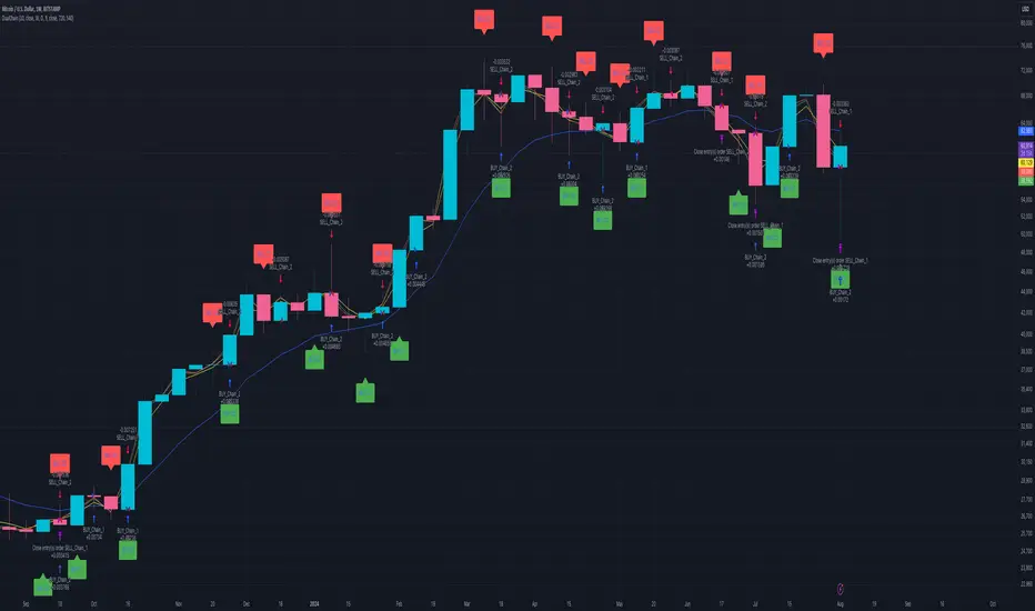
Filtered MACD with Backtest [UAlgo]The "Filtered MACD with Backtest " indicator is an advanced trading tool designed for the TradingView platform. It combines the Moving Average Convergence Divergence (MACD) with additional filters such as Moving Average (MA) and Average Directional Index (ADX) to enhance trading signals. This indicator aims to provide more reliable entry and exit points by filtering out noise and confirming trends. Additionally, it includes a comprehensive backtesting module to simulate trading strategies and assess their performance based on historical data. The visual backtest module allows traders to see potential trades directly on the chart, making it easier to evaluate the effectiveness of the strategy.
🔶 Customizable Parameters :
Price Source Selection: Users can choose their preferred price source for calculations, providing flexibility in analysis.
Filter Parameters:
MA Filter: Option to use a Moving Average filter with types such as EMA, SMA, WMA, RMA, and VWMA, and a customizable length.
ADX Filter: Option to use an ADX filter with adjustable length and threshold to determine trend strength.
MACD Parameters: Customizable fast length, slow length, and signal smoothing for the MACD indicator.
Backtest Module:
Entry Type: Supports "Buy and Sell", "Buy", and "Sell" strategies.
Stop Loss Types: Choose from ATR-based, fixed point, or X bar high/low stop loss methods.
Reward to Risk Ratio: Set the desired take profit level relative to the stop loss.
Backtest Visuals: Display entry, stop loss, and take profit levels directly on the chart with
colored backgrounds.
Alerts: Configurable alerts for buy and sell signals.
🔶 Filtered MACD : Understanding How Filters Work with ADX and MA
ADX Filter:
The Average Directional Index (ADX) measures the strength of a trend. The script calculates ADX using the user-defined length and applies a threshold value.
Trading Signals with ADX Filter:
Buy Signal: A regular MACD buy signal (crossover of MACD line above the signal line) is only considered valid if the ADX is above the set threshold. This suggests a stronger uptrend to potentially capitalize on.
Sell Signal: Conversely, a regular MACD sell signal (crossunder of MACD line below the signal line) is only considered valid if the ADX is above the threshold, indicating a stronger downtrend for potential shorting opportunities.
Benefits: The ADX filter helps avoid whipsaws or false signals that might occur during choppy market conditions with weak trends.
MA Filter:
You can choose from various Moving Average (MA) types (EMA, SMA, WMA, RMA, VWMA) for the filter. The script calculates the chosen MA based on the user-defined length.
Trading Signals with MA Filter:
Buy Signal: A regular MACD buy signal is only considered valid if the closing price is above the MA value. This suggests a potential uptrend confirmed by the price action staying above the moving average.
Sell Signal: Conversely, a regular MACD sell signal is only considered valid if the closing price is below the MA value. This suggests a potential downtrend confirmed by the price action staying below the moving average.
Benefits: The MA filter helps identify potential trend continuation opportunities by ensuring the price aligns with the chosen moving average direction.
Combining Filters:
You can choose to use either the ADX filter, the MA filter, or both depending on your strategy preference. Using both filters adds an extra layer of confirmation for your signals.
🔶 Backtesting Module
The backtesting module in this script allows you to visually assess how the filtered MACD strategy would have performed on historical data. Here's a deeper dive into its features:
Backtesting Type: You can choose to backtest for buy signals only, sell signals only, or both. This allows you to analyze the strategy's effectiveness in different market conditions.
Stop-Loss Types: You can define how stop-loss orders are placed:
ATR (Average True Range): This uses a volatility measure (ATR) multiplied by a user-defined factor to set the stop-loss level.
Fixed Point: This allows you to specify a fixed dollar amount or percentage value as the stop-loss.
X bar High/Low: This sets the stop-loss at a certain number of bars (defined by the user) above/below the bar's high (for long positions) or low (for short positions).
Reward-to-Risk Ratio: Define the desired ratio between your potential profit and potential loss on each trade. The backtesting module will calculate take-profit levels based on this ratio and the stop-loss placement.
🔶 Disclaimer:
Use with Caution: This indicator is provided for educational and informational purposes only and should not be considered as financial advice. Users should exercise caution and perform their own analysis before making trading decisions based on the indicator's signals.
Not Financial Advice: The information provided by this indicator does not constitute financial advice, and the creator (UAlgo) shall not be held responsible for any trading losses incurred as a result of using this indicator.
Backtesting Recommended: Traders are encouraged to backtest the indicator thoroughly on historical data before using it in live trading to assess its performance and suitability for their trading strategies.
Risk Management: Trading involves inherent risks, and users should implement proper risk management strategies, including but not limited to stop-loss orders and position sizing, to mitigate potential losses.
No Guarantees: The accuracy and reliability of the indicator's signals cannot be guaranteed, as they are based on historical price data and past performance may not be indicative of future results.

Fractal Breakout Trend Following StrategyOverview
The Fractal Breakout Trend Following Strategy is a trend-following system which utilizes the Willams Fractals and Alligator to execute the long trades on the fractal's breakouts which have a high probability to be the new uptrend phase beginning. This system also uses the normalized Average True Range indicator to filter trades after a large moves, because it's more likely to see the trend continuation after a consolidation period. Strategy can execute only long trades.
Unique Features
Trend and volatility filtering system: Strategy uses Williams Alligator to filter the counter-trend fractals breakouts and normalized Average True Range to avoid the trades after large moves, when volatility is high
Configurable Trading Periods: Users can tailor the strategy to specific market windows, adapting to different market conditions.
Flexible Risk Management: Users can choose the stop-loss percent (by default = 3%) for trades, but strategy also has the dynamic stop-loss level using down fractals.
Methodology
The strategy places stop order at the last valid fractal breakout level. Validity of this fractal is defined by the Williams Alligator indicator. If at the moment of time when price breaking the last fractal price is higher than Alligator's teeth line (8 period SMA shifted 5 bars in the future) this is a valid breakout. Moreover strategy has the additional volatility filtering system using normalized ATR. It calculates the average normalized ATR for last user-defined number of bars and if this value lower than the user-defined threshold value the long trade is executed.
When trade is opened, script places the stop loss at the price higher of two levels: user defined stop-loss from the position entry price or down fractal validation level. The down fractal is valid with the rule, opposite as the up fractal validation. Price shall break to the downside the last down fractal below the Willians Alligator's teeth line.
Strategy has no fixed take profit. Exit level changes with the down fractal validation level. If price is in strong uptrend trade is going to be active until last down fractal is not valid. Strategy closes trade when price hits the down fractal validation level.
Risk Management
The strategy employs a combined approach to risk management:
It allows positions to ride the trend as long as the price continues to move favorably, aiming to capture significant price movements. It features a user-defined stop-loss parameter to mitigate risks based on individual risk tolerance. By default, this stop-loss is set to a 3% drop from the entry point, but it can be adjusted according to the trader's preferences.
Justification of Methodology
This strategy leverages Williams Fractals to open long trade when price has broken the key resistance level to the upside. This resistance level is the last up fractal and is shall be broken above the Williams Alligator's teeth line to be qualified as the valid breakout according to this strategy. The Alligator filtering increases the probability to avoid the false breakouts against the current trend.
Moreover strategy has an additional filter using Average True Range(ATR) indicator. If average value of ATR for the last user-defined number of bars is lower than user-defined threshold strategy can open the long trade according to open trade condition above. The logic here is following: we want to open trades after period of price consolidation inside the range because before and after a big move price is more likely to be in sideways, but we need a trend move to have a profit.
Another one important feature is how the exit condition is defined. On the one hand, strategy has the user-defined stop-loss (3% below the entry price by default). It's made to give users the opportunity to restrict their losses according to their risk-tolerance. On the other hand, strategy utilizes the dynamic exit level which is defined by down fractal activation. If we assume the breaking up fractal is the beginning of the uptrend, breaking down fractal can be the start of downtrend phase. We don't want to be in long trade if there is a high probability of reversal to the downside. This approach helps to not keep open trade if trend is not developing and hold it if price continues going up.
Backtest Results
Operating window: Date range of backtests is 2023.01.01 - 2024.05.01. It is chosen to let the strategy to close all opened positions.
Commission and Slippage: Includes a standard Binance commission of 0.1% and accounts for possible slippage over 5 ticks.
Initial capital: 10000 USDT
Percent of capital used in every trade: 30%
Maximum Single Position Loss: -3.19%
Maximum Single Profit: +24.97%
Net Profit: +3036.90 USDT (+30.37%)
Total Trades: 83 (28.92% win rate)
Profit Factor: 1.953
Maximum Accumulated Loss: 963.98 USDT (-8.29%)
Average Profit per Trade: 36.59 USDT (+1.12%)
Average Trade Duration: 72 hours
These results are obtained with realistic parameters representing trading conditions observed at major exchanges such as Binance and with realistic trading portfolio usage parameters.
How to Use
Add the script to favorites for easy access.
Apply to the desired timeframe and chart (optimal performance observed on 4h and higher time frames and the BTC/USDT).
Configure settings using the dropdown choice list in the built-in menu.
Set up alerts to automate strategy positions through web hook with the text: {{strategy.order.alert_message}}
Disclaimer:
Educational and informational tool reflecting Skyrex commitment to informed trading. Past performance does not guarantee future results. Test strategies in a simulated environment before live implementation

Fine-Tune Inputs: Fourier Smoothed Hybrid Volume Spread AnalysisUse this Strategy to Fine-tune inputs for the HSHVSA Indicator.
Strategy allows you to fine-tune the indicator for 1 TimeFrame at a time; cross Timeframe Input fine-tuning is done manually after exporting the chart data.
I suggest using " Close all " input False when fine-tuning Inputs for 1 TimeFrame. When you export data to Excel/Numbers/GSheets I suggest using " Close all " input as True , except for the lowest TimeFrame.
MEANINGFUL DESCRIPTION:
The Fourier Smoothed Hybrid Volume Spread Analysis (FSHVSA) Strategy/Indicator is an innovative trading tool designed to fuse volume analysis with trend detection capabilities, offering traders a comprehensive view of market dynamics.
This Strategy/Indicator stands apart by integrating the principles of the Discrete Fourier Transform (DFT) and volume spread analysis, enhanced with a layer of Fourier smoothing to distill market noise and highlight trend directions with unprecedented clarity.
This smoothing process allows traders to discern the true underlying patterns in volume and price action, stripped of the distractions of short-term fluctuations and noise.
The core functionality of the FSHVSA revolves around the innovative combination of volume change analysis, spread determination (calculated from the open and close price difference), and the strategic use of the EMA (default 10) to fine-tune the analysis of spread by incorporating volume changes.
Trend direction is validated through a moving average (MA) of the histogram, which acts analogously to the Volume MA found in traditional volume indicators. This MA serves as a pivotal reference point, enabling traders to confidently engage with the market when the histogram's movement concurs with the trend direction, particularly when it crosses the Trend MA line, signalling optimal entry points.
It returns 0 when MA of the histogram and EMA of the Price Spread are not align.
WHAT IS FSHVSA INDICATOR:
The FSHVSA plots a positive trend when a positive Volume smoothed Spread and EMA of Volume smoothed price is above 0, and a negative when negative Volume smoothed Spread and EMA of Volume smoothed price is below 0. When this conditions are not met it plots 0.
HOW TO USE THE STRATEGY:
Here you fine-tune the inputs until you find a combination that works well on all Timeframes you will use when creating your Automated Trade Algorithmic Strategy. I suggest 4h, 12h, 1D, 2D, 3D, 4D, 5D, 6D, W and M.
ORIGINALITY & USEFULNESS:
The FSHVSA Strategy is unique because it applies DFT for data smoothing, effectively filtering out the minor fluctuations and leaving traders with a clear picture of the market's true movements. The DFT's ability to break down market signals into constituent frequencies offers a granular view of market dynamics, highlighting the amplitude and phase of each frequency component. This, combined with the strategic application of Ehler's Universal Oscillator principles via a histogram, furnishes traders with a nuanced understanding of market volatility and noise levels, thereby facilitating more informed trading decisions.
DETAILED DESCRIPTION:
My detailed description of the indicator and use cases which I find very valuable.
What is the meaning of price spread?
In finance, a spread refers to the difference between two prices, rates, or yields. One of the most common types is the bid-ask spread, which refers to the gap between the bid (from buyers) and the ask (from sellers) prices of a security or asset.
We are going to use Open-Close spread.
What is Volume spread analysis?
Volume spread analysis (VSA) is a method of technical analysis that compares the volume per candle, range spread, and closing price to determine price direction.
What does this mean?
We need to have a positive Volume Price Spread and a positive Moving average of Volume price spread for a positive trend. OR via versa a negative Volume Price Spread and a negative Moving average of Volume price spread for a negative trend.
What if we have a positive Volume Price Spread and a negative Moving average of Volume Price Spread?
It results in a neutral, not trending price action.
Thus the Indicator/Strategy returns 0 and Closes all long and short positions.
In the next Image you can see that trend is negative on 4h, we just move Negative on 12h and Positive on 1D. That means trend/Strategy flipped negative .
I am sorry, the chart is a bit messy. The idea is to use the indicator/strategy over more than 1 Timeframe.
Use this Strategy to fine-tune inputs for the HSHVSA Indicator.
(Strategy allows you to fine-tune the indicator for 1 TimeFrame at a time; cross Timeframe Input fine-tuning is done manually after exporting the chart data)
I suggest using " Close all " input False when fine-tuning Inputs for 1 TimeFrame. When you export data to Excel/Numbers/GSheets I suggest using " Close all " input as True , except for the lowest TimeFrame. I suggest using 100% equity as your default quantity for fine-tune purposes. I have to mention that 100% equity may lead to unrealistic backtesting results. Be avare. When backtesting for trading purposes use Contracts or USDT.
